 Applied Mathematics, 2013, 4, 1526-1530 Published Online November 2013 (http://www.scirp.org/journal/am) http://dx.doi.org/10.4236/am.2013.411206 Open Access AM Algorithms for Computing Some Invariants for Discrete Knots Gabriela Hinojosa, David Torres, Rogelio Valdez Facultad de Ciencias, Universidad Autónoma del Estado de Morelos, Cuernavaca, México Email: gabriela@uaem.mx, david.tormor@gmail.com, valdez@uaem.mx Received April 18, 2013; revised May 18, 2013; accepted May 25, 2013 Copyright © 2013 Gabriela Hinojosa et al. This is an open access article distributed under the Creative Commons Attribution Li- cense, which permits unrestricted use, distribution, and reproduction in any medium, provided the original work is properly cited. ABSTRACT Given a cubic knot K, there exists a projection of the Euclidean space onto a suitable plane such that p(K) is a knot diagram and it can be described in a discrete way as a cycle permutation. Using this fact, we develop an algorithm for computing some invariants for K: its fundamental group, the genus of its Seifert surface and its Jones polynomial. 3 :pP3 3 P Keywords: Cubic Knots; Discrete Knots; Algorithms 1. Introduction Considering the set consists of the lattice and all the straight lines parallel to the coordinate axis and passing through points in , we say that a knot 3 S3 3 3 is a cubic knot if it is contained in . In [1] it was shown that any classical knot is isotopic to a cubic knot and by [2] we know that there exists a generic pro- jection p of any cubic knot into a suitable plane. If we combine these two results, we have that p(K) is a dia- gram of K and it can be described in a discrete way as a cyclic permutation of points S ,,, n w 12 ww (with some restrictions). This allows us to develop an algorithm for computing the fundamental group of K, the genus of its Seifert surface and its Jones polynomial. 2. Discrete Knots and Some Invariants Consider an oriented cubic knot K. In [2] it was proved that we can associate to K a unique sequence of points such that , ij , 12 ,, , n v v v 3 i vvv1,ij n , i is joined to 1i by a unit edge, n v is likewise joined to 1 by a unit edge, and the numbering of the i’s is compatible with the orientation of K. Henceforth, we will assume that all the coordinates of the points in K are positive. v v v v An advantage of cubic knots is that there exists a ca- nonical generic projection p (for details see [2]). In fact, let , where is the well-known tran- scendental number. Let P be the plane through the origin in orthogonal to N and consider the orthogonal pro- jection . Then 2 1, π,πN P π 3 3 :p3 p is injective. Let ˆ pK be its projection into the plane P. Thus ˆ is a polygonal curve contained in P with some self-in- tersections called inessential vertices or crossings. The crossings are not contained in 3:P pp K and are transverse, hence p is regular. The projections of the vertices of K are contained in , and are called verti- ces. Hence we can write ˆ as a cyclic permutation of points 12 ,,,ww w n n where iP , ij , w ww 1,ij w and i is joined to 1i by a straight line segment whose preimage is a unit edge and in the same way is likewise joined to (for details see [2]). w w n1 Definition 2.1. A discrete knot K ̂ is the equivalence class of the n cyclic permutations of n points w ,,, n w 12 in P ww P such that the ’s satisfy the above assumptions. i w ˆ Next we will describe the crossings of . Consider an orthonormal basis β of the plane , given by 3 P 23 2 π,π,1 π 11 0, AB π,1, where 2 π1A and 246 2π2ππ1B w 4 ˆ i wK . Con- sider four points 1 i, 2 i, 3 i and whose coordinates with respect to the basis β are w w y, j ijj . The following lemma gives us a criteria to know when the line segment wx 12 iiintersects the line segment ww 34 ii . Notice that for the computing algorithm purpose, we just need to consider only the quadruples of points ww 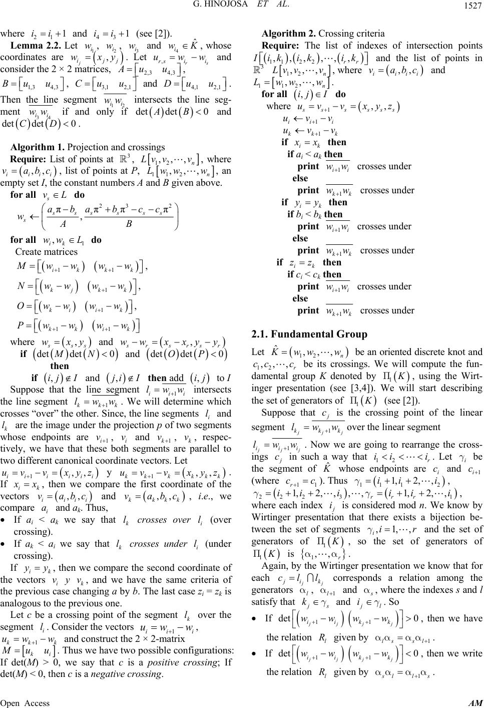 G. HINOJOSA ET AL. 1527 where and (see [2]). 21 43 Lemma 2.2. Let 3 i and , whose coordinates are j ij . Let rs and consider the 2 × 2 matrices, , 1ii 1,3 4,3 u 1ii 1 i, 2 i w, w ,j wxy 3,1 2,1 Cu u w 4 ˆ i wK i uw 4,3 u Du ,rs i w 32, Au Bu, and . 4,12,1 u Then the line segment 12 ii intersects the line seg- ment ww 34 ii ww if and only if det det0AB and . detC det 0D Algorithm 1. Projection and crossings Require: List of points at , 3 12 ,,, n Lv vv , where , list of points at P, ,, iiii vabc 112 ,,Lww, n w, an empty set I, the constant numbers A and B given above. for all do s vL 23 2 πππ π , ssss ss s ababcc w AB for all do 1 Create matrices , ik ww L , 11ik kk Mwwww , 1kjk k Nww ww , 1kiik Owwww 11kk ik Pww ww where , ss wxy and , rsrsr wwxxy y if and det detMN 0 det det0OP then if and ,ijI,jiI then add ,ij to I Suppose that the line segment 1iii lw intersects the line segment w 1kkk. We will determine which crosses “over” the other. Since, the line segments i and k are the image under the projection p of two segments whose endpoints are 1i, i and 1k, k, respec- tively, we have that these both segments are parallel to two different canonical coordinate vectors. Let y 1kk k kkk . If i lww l ,,y l v i z vv v v x 1,, ii i ii uv v xy k uv z x ,, ii vab a , then we compare the first coordinate of the vectors ii and , i.e., we compare and ak. Thus, c ,, k b kk vak c i If ai < ak we say that k l crosses over i l (over crossing). If ak < ai we say that k l crosses under i l (under crossing). If ik , then we compare the second coordinate of the vectors i y k, and we have the same criteria of the previous case changing a by b. The last case zi = zk is analogous to the previous one. yy v v Let c be a crossing point of the segment over the segment . Consider the vectors 1iii, and construct the 2 × 2-matrix k l w i l 1 uw kk uw w k ki uu. Thus we have two possible configurations: If det(M) > 0, we say that c is a positive crossing; If det(M) < 0, then c is a negative crossing. Algorithm 2. Crossing criteria Require: The list of indexes of intersection points 112 2 ,,,,,, rr ik ikik 3 and the list of points in 12 ,,, n Lv vv, where and ,, iiii vabc 112 ,,, n Lwww. for all ,ijI do where 1,, sssss v xyz uvv uv 1iii 1kk v k uv if ik x then if ai < ak then print 1ii ww crosses under else print 1kk ww crosses under if ik yy then if bi < bk then print 1ii ww crosses under else print 1kk ww crosses under if ik zz then if ci < ck then print 1ii ww crosses under else print 1kk ww crosses under 2.1. Fundamental Group Let 12 ˆ,,, n ww w ,,, r c be an oriented discrete knot and 12 be its crossings. We will compute the fun- damental group K denoted by cc 1 P, using the Wirt- inger presentation (see [3,4]). We will start describing the set of generators of 1 P (see [2]). Suppose that c is the crossing point of the linear segment 1 j kk lww j k over the linear segment 1 jj iii ings lww. Now we are going to rearrange the cross- c in such a way that 12 r. Let i be the segment of ii i g ˆ whose endpoints are and i c1i c (where 1r c 1 c ). Thus , 11 1 1,2, ,ii 2 ig ,i 22 2 31 , where each index 1, 2ii, ,,, gg1, 2, rr r iii i is considered mod n. We know by Wirtinger presentation that there exists a bijection be- tween the set of segments and the set of generators of ,1,, iirg 1 P, so the set of generators of 1 P is 1,,aa r Again, by the Wirtinger presentation we know that for each . j ik cll l al corresponds a relation among the generators , 1 a and a, where the indexes s and l satisfy that s k g and l ig. So If 11 det 0 jjj j iikk ww ww , then we have the relation given by . l R1ls sl aa aa If 11 det 0 jjj j iikk ww ww , then we write the relation given by l R1 ll aaa a s . Open Access AM 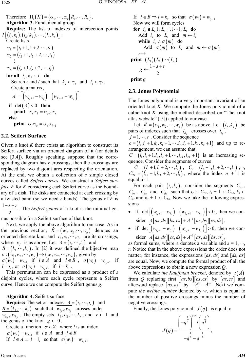 G. HINOJOSA ET AL. 1528 Therefore 111 ,, ,, rr RRPaa. Algorithm 3. Fundamental group Require: The list of indexes of intersection points 112 2 ,,, ,,, rr ikikik . Create lists 11 12 22 23 1 1,2,, 1,2, , 1,2,, rr r ii i ii i ii i g g g for all do , jj ik L Search r and l such that s kg and l ig. Create a matrix, 11 jjjj ii kk Aw www if then det 0A print 1 ll aa s aa else print 1ls sl aa aa 2.2. Seifert Surface Given a knot K there exists an algorithm to construct its Seifert surface via an oriented diagram of it (for details see [3,4]). Roughly speaking, suppose that the corre- sponding diagram has r crossings, then the crossings are replaced by two disjoint arcs respecting the orientation. At the end, we obtain a collection of s simple closed curves called Seifert curves. We construct a Seifert sur- face F for K considering each Seifert curve as the bound- ary of a disk. The disks are connected at each crossing by a twisted band (so we need r bands). The genus of F is 1 2 r. The Seifert genus of a knot is the minimal ge- nus possible for a Seifert surface of that knot. Next, we apply the above algorithm to our case. As in the previous section, 12 ˆ,,, n ww w 12 ,,, r cc c denotes an oriented discrete knot and are its crossings, where c is as above. Let 1r ii,, 12 ,,, nn ww w AlB and . In [2] it was defined the bijective map , given by if and , 1,, 12 :,ww ll r Bk k ,,s 1 ww s w l 1 s lk ww s if li s, or if 1 s li ww lk . This permutation can be expressed as a product of s disjoint cycles, where each cycle represents a Seifert curve. Hence we can compute the Seifert genus g. Algorithm 4. Seifert surface Require: The set or indexes 1,, r ii and such that 1,, r Bk k 1 j i w i w crosses under 1 j kk . The empty sets , and ww 12 ,,, n LLL 1r and the genus of the knot . 0g Create a function where l is an index if and lB 1ll ww slA If lA li so that w1 s lk w s If lB lk so that 1 s li ww s Now we will form cycles for 11srr iLL L do Add i L to and r mi while s im do Add m to and r L mm r++ print 12 r LL L 2 r1 g print g 2.3. Jones Polynomi al The Jones polynomial is a very important invariant of an oriented knot K. We compute the Jones polynomial of a cubic knot K using the method described on “The knot atlas website” ([5]) applied to our case. Let 12 ˆ,,, n ww w be as above. Let , j ik be pairs of indexes such that k crosses over l i l, 1,j,r . Consider the sequence 1,,1 r r kk 111 1 ,1,,1,, rr i kki,ici and up to re- arrangement, we can assume that 1 112 22 ,1,, 1,,l lll2 , kk lCl is an increasing se- quence. Consider the segments of curves 11 12 1,2, ,Cl ll , ,···, 22 23 1,2,,Cl ll 22 2 1,2,, kk k Cl l 1 l, where the index n + 1 is equal to 1. For each pair , s ik , consider the segments as , , cs and ds such that is Ccs, is + 1 Cas, ks Cds and ks + 1 Cbs. Now we take the following expres- sions C bs C CC If 11 det 0 ssss ii kk wwww , then we con- sider 1 ,, ,, as dsbscsAasbscsds, if 0wwww 11 det ssss ii kk , then we con- sider 1 ,, ,, as dscsdsAas dsbscs, as formal sums, where A denotes a variable and s = 1, ···, r. Notice that in the above expressions the order does not matter; for instance, the expressions [as, ds] and [ds, as] are equal. Now, we compute the formal product of all the above expressions to obtain a new expression Q. We calculate the Kauffman bracket, denoted by tA from Q replacing first ,,as bsbs cs by ,as cs and afterward replace ,as as2 by 2 A . Next we com- pute the writhe number denoted by w, which is equal to the number of positive crossings minus the number of negative crossings. Finally, the Jones polynomial q is equal to 1 3 1 44 11 22 w qt J q q q q , Open Access AM 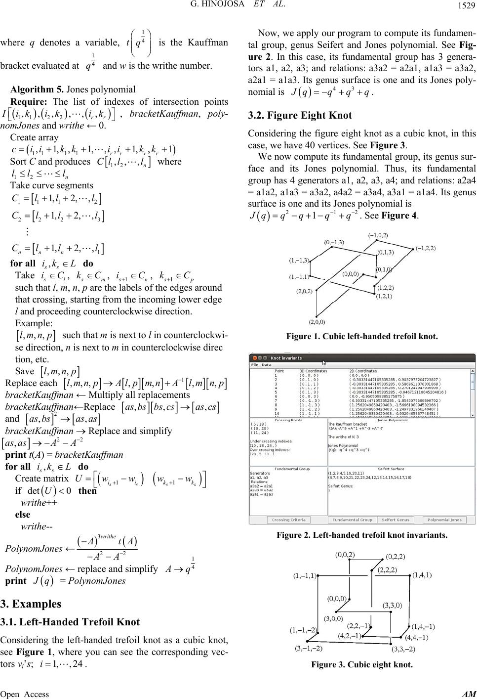 G. HINOJOSA ET AL. 1529 where q denotes a variable, 1 4 tq is the Kauffman bracket evaluated at 1 4 q and w is the writhe number. Algorithm 5. Jones polynomial Require: The list of indexes of intersection points 112 2 ,,, ,,, rr ikikik , bracketKauffman, poly- nomJones and writhe ← 0. Create array 111 1 ,1,,1,, ,1,,1 rrr r cii kkiikk Sort C and produces 12 n ,, ,Clll where 12 n Take curve segments ll l 11 12 22 23 1 1,2, , 1,2,, 1,2, , nn n Cl ll Cl ll Cl ll for all do , ss ik L Take l iC, m1 kC, n1 iC , p such that l, m, n, p are the labels of the edges around kC that crossing, starting from the incoming lower edge l and proceeding counterclockwise direction. Example: ,,,lmnp such that m is next to l in counterclockwi- se direction, n is next to m in counterclockwise direc tion, etc. Save ,,,lmnp Replace each 1 ,,,, ,npAlp mnAlmnp ,,lm bracketKauffman ← Multiply all replacements bracketKauffman←Replace ,, ,as bsbs csas cs and 2 ,,as bsas as bracketKauffman Replace and simplify 22 ,as as A print t(A) = bracketKauffman for all do , ss ik L Create matrix 11 ssss ii kk Uwww w if then det 0U writhe++ else writhe-- PolynomJones ← 3 22 writhe tA AA PolynomJones ← replace and simplify 1 4 q print q = PolynomJones 3. Examples 3.1. Left-Handed Trefoil Knot Considering the left-handed trefoil knot as a cubic knot, see Figure 1, where you can see the corresponding vec- tors vi’s; . 1,,24i Now, we apply our program to compute its fundamen- tal group, genus Seifert and Jones polynomial. See Fig- ure 2. In this case, its fundamental group has 3 genera- tors a1, a2, a3; and relations: a3a2 = a2a1, a1a3 = a3a2, a2a1 = a1a3. Its genus surface is one and its Jones poly- nomial is 43 qqqJq . 3.2. Figure Eight Knot Considering the figure eight knot as a cubic knot, in this case, we have 40 vertices. See Figure 3. We now compute its fundamental group, its genus sur- face and its Jones polynomial. Thus, its fundamental group has 4 generators a1, a2, a3, a4; and relations: a2a4 = a1a2, a1a3 = a3a2, a4a2 = a3a4, a3a1 = a1a4. Its genus surface is one and its Jones polynomial is 21 1qqq qJq 2 . See Figure 4. Figure 1. Cubic left-handed trefoil knot. Figure 2. Left-handed trefoil knot invariants. Figure 3. Cubic eight knot. Open Access AM  G. HINOJOSA ET AL. Open Access AM 1530 REFERENCES [1] M. Boege, G. Hinojosa and A. Verjovsky, “Any Smooth Knot Sn ℝn+2 Is Isotopic to a Cubic Knot Contained in the Canonical Scaffolding of n+2,” Revista Matemática Complutense, Vol. 24, No. 1, 2011, pp. 1-13. http://dx.doi.org/10.1007/s13163-010-0037-4 [2] G. Hinojosa, A. Verjovsky and C. V. Marcotte, “Cubu- lated Moves and Discrete Knots,” 2013, pp. 1-40. http://arxiv.org/abs/1302.2133 [3] D. Rolfsen, “Knots and Links,” AMS Chelsea Publishing, American Mathematical Society, Providence Rhode Is- land, 2003. [4] R. H. Fox, “A Quick Trip through Knot Theory. Topol- ogy of 3-Manifolds and Related Topics,” Prentice-Hall, Inc., Upper Saddle River, 1962. [5] “The Knot Atlas,” 2013. http://katlas.math.toronto.edu Figure 4. Figure eight knot invariants. 4. Acknowledgements Gabriela Hinojosa thanks CONACyT (México), for its financial support CB-2009-129939 and all the authors thank PROMEP (México) for supporting the publication of this paper.
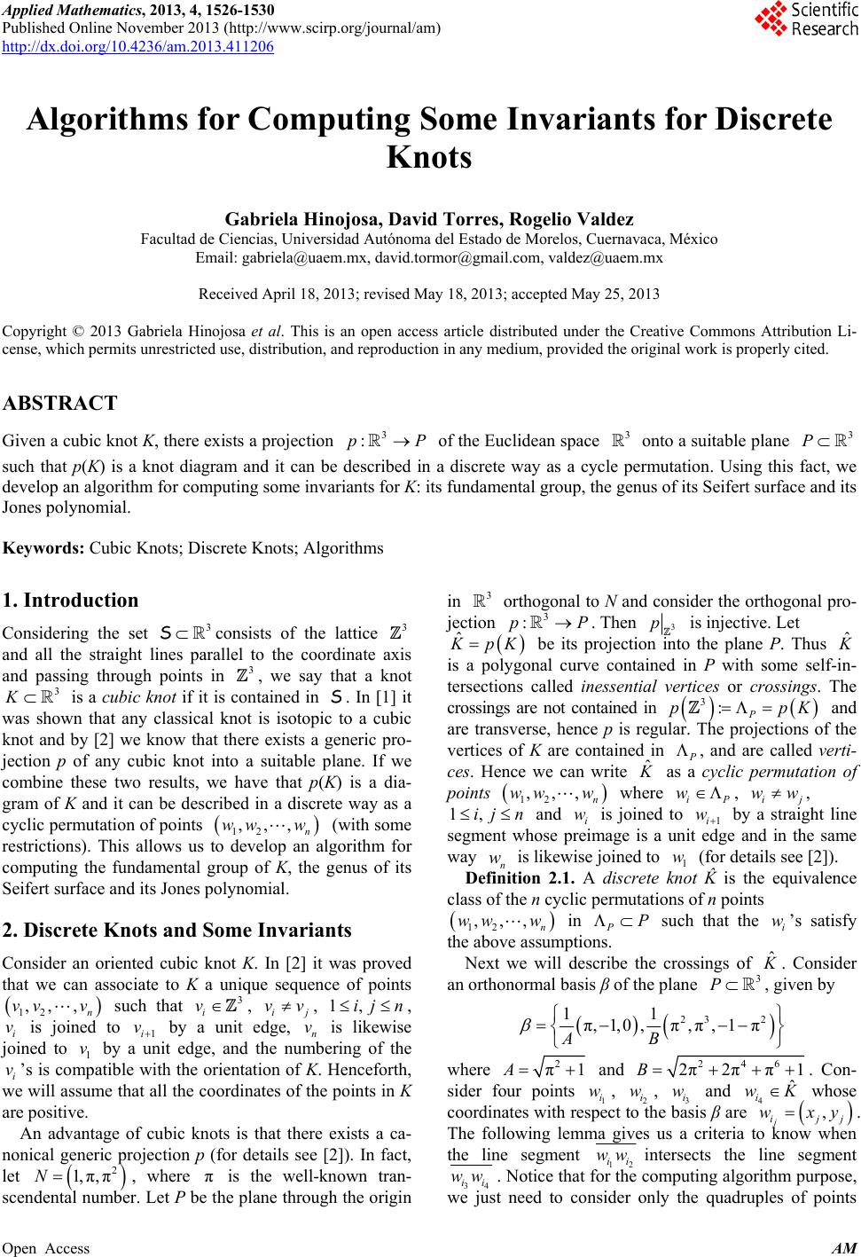
|