Journal of Signal and Information Processing, 2013, 4, 375-384
Published Online November 2013 (http://www.scirp.org/journal/jsip)
http://dx.doi.org/10.4236/jsip.2013.44048
Open Access JSIP
375
Contribution in Information Signal Processing for Solving
State Space Nonlinear Estimation Problems
Hamza Benzerrouk1*, Alexander Nebylov2, Hassen Salhi1*
1SET Laboratory (Systèmes Electriques et Télecommande) of Electronic, Department of Saad Dahlab, University of Blida, Blida,
Algeria; 2International Institute for Advanced Aerospace Technologies, Saint-Petersburg State University of Aerospace Instrumenta-
tion, Saint Petersburg, Russia.
Received May 12th, 2013; revised September 30th, 2013; accepted October 8th, 2013
Copyright © 2013 Hamza Benzerrouk et al. This is an open access article distributed under the Creative Commons Attribution Li-
cense, which permits unrestricted use, distribution, and reproduction in any medium, provided the original work is properly cited.
ABSTRACT
In this paper, comprehensive methods to apply several formulations of nonlinear estimators to integrated navigation
problems are considered and developed. The problem of linear and nonlinear filters such as Kalman Filter (KF) and
Extended Kalman Filter (EKF) is stated. Analog solution which is based on fisher information matrix propagation for
linear and nonlinear filtering is also developed. Additionally, the idea of iterations is included through the update step
both for Kalman filters and Information filters in order to improve accuracy. Through this development, two new for-
mulations of High order Kalman filters and High order Information filters are presented. Finally, in order to compare
these different nonlinear filters, special applications are analyzed by using the proposed techniques to estimate two
well-known mathematical state space models, which are based on nonlinear time series used to apply these estimation
algorithms. A criterion used for comparison is the root mean square error RMSE and several simulations under specific
conditions are illustrated.
Keywords: Kalman Filter; Information Filter; Extended Kalman Filter; Extended Information Filter; 2nd Order Kalman
Filter; 2nd Order Information Filter
1. Introduction
Different kinds of filters exist and were developed in
order to ensure high quality measurement in input-output
systems and permit more accurate control system in sev-
eral fields such as in Aerospace, for aircraft’s navigation,
ship, spacecraft, tracking etc. Kalman filter (KF) was
firstly derived from using orthogonality principle and pre-
sented in [1-3]. Generally so-called filter or/and estima-
tor, is/are one of several techniques of estimation based
on LMMSE (Linear Minimum Mean Square Error) [4].
In 1970, Kalman and Bucy introduced extended Kalman
filter for nonlinear estimation. Actually this kind of filter
is called standard local filter and is based on approxima-
tion of nonlinear functions by Taylor series. The most
common filter in the field of engineering and aerospace
especially, is the extended Kalman filter. These local
standard filters also contain the second order Kalman
filter and the iterated filter. Other kinds of nonlinear
filtering algorithms exist but are not treated in this paper
[5]. The most interesting and main idea introduced in this
paper is to use the parallel solutions to Kalman filter and
standard local filters which are based on the Fisher In-
formation Matrix propagation [6,7]. It is analog to Kal-
man technique but is more efficient and robust to several
constraints. The main idea is to use the inverse matrix
lemma to develop analog estimator to Kalman filter with
less computational time. These filters are more efficient
when the number of the input is more than the dimension
of the state vector. In this paper, we introduced classic
information filters for linear and nonlinear filtering
problem. Behind this was explored in our solution, the
efficiency includes iterations through the updated step of
the different algorithms [8]. Two new formulations are
presented such as the iterated second order Kalman filter
and the second order information filter followed by the
second order Iterated Information filter. So, generally the
step of initialization is the main important in nonlinear
filtering and we propose to use the information filters to
*Corresponding authors.

Contribution in Information Signal Processing for Solving State Space Nonlinear Estimation Problems 376
solve the problem of initialization. Of course, informa-
tion filters present several other advantages when the
state space model input is a combination of several sen-
sors as in data fusion or multi-sensors fusion, it was
proven that comparing with Kalman filter and extended
Kalman filter both for linear and nonlinear case, the in-
formation filters are more easy to implement in real time
application with multiple information combination [9-12].
We apply these different nonlinear filters to dynamical
state models such as references. It is expected that this
work could serve in investigate integrated navigation
system INS (Inertial navigation System)/GNSS (Global
Navigation by Satellite System) problems, in order to
show possible application in the field of aerospace.
2. Kalman Filter and Nonlinear Filtering
If the system is linear and the statistical distribution is
Gaussian, then the Bayesian prediction and update equa-
tion can be solved analytically. The system is completely
described by the Gaussian parameters such as mean and
covariance and this filter is called the Kalman filter [13].
As a discrete statistical recursive algorithm, Kalman fil-
ter provides an estimate of the state at time k given all
observations up to time k and provides an optimal mini-
mal mean squared error estimate of these states.
Process Model: A linear dynamic system in discrete
time can be described by
1.0
.
kkkk
kkkk
xFxw
k
zHxv



 (1)
Kalman filter is usually called as the optimal filter in the
case of linear assumption and white Gaussian noises both
in state and in measurement equations.
2.1. Extended Kalman Filter
In most real applications the process and/or observation
models are nonlinear and hence linear Kalman filter al-
gorithm described above cannot be directly applied. To
overcome this, a linearised Kalman filter or Extended
Kalman Filter (EKF) can be applied which are estimators
where the models are continuously linearized before ap-
plying the estimation techniques [14].
However, in most practical navigation applications,
nominal trajectory does not exist beforehand. The solu-
tion is to use the current estimated state from the filter at
each time step k as the linearization reference from which
the estimation procedure can proceed. Such algorithm is
called extended Kalman filter. If the filter operates prop-
erly, the linearization error around the estimated solution
can be maintained at a reasonably small value [15-17].
However, if the filter is ill-conditioned due to modeling
errors, incorrect tuning of the covariance matrices, or
initialization error, then the estimation error will affect
the linearization error which in turn will affect the esti-
mation process and is known as filter divergence. For
this reason the EKF requires greater care in modeling and
tuning than the linear Kalman filter. Let us describe bel-
low the algorithm of EKF [18]: based on state space
model as:



1.0
.
kkkk
kkk k
xfxw
k
zhx v






(2)
and on the linearization using taylor approximation at the
first order we get the state space model given in [19].


k
F

is the Jacobian matrix of and

k
f


k
H

is
the Jacobian matrix of


k
h

.
Initialization:
0
ˆ
x
et . (3)
0
P
Prediction:


 
1/
T
/1 1
ˆˆ
ˆˆ
kkk k
kkkkk kkk
xfx
PFxPFx



Q

 (4)
Update:
 



TT
/1/1/1 /1/1
1
/1 /1
/1/1 /1
ˆˆ ˆ
ˆˆ ˆ
ˆ
1;
k kkkkkkkkkkkkk
k
kkk kkkkk
kkkkkkkkk
KPHxHx PHx
R
xx KZhx
PPKHxP
KK
 






  




(5)
The meaning of the extended Kalman filter can be un-
derstudied by appreciating the same equation of gain
calculation as in the Kalman filter at the difference that
in the nonlinear filtering, EKF is sub-optimal filter.
2.2. Iterated Filter
One can distinguish the importance of the two different
steps; prediction and update, it allows to observe the ef-
fect of new information given by the measurements in
the filtering step. Let us focus on the estimation of the
mean and the covariance of the state vector. In Equation
(5) it is clear that ˆk
x
contains more information about
k
x
than ˆk
x

. Nonetheless, the linearization was made in
ˆk
x

. This fact is used and the linearization can be made in
the kth step again but this time in ˆk
x
. This provides a
new value of estimates and such a procedure may be re-
peated as long as a difference between two subsequent
estimates is lower than a specified

. Thus, the follow-
ing equations will be implemented using the iterated
form: 1
ˆˆ
kk
x
x

and 1
k
PP
k

; For 1,2, 3,i
Open Access JSIP

Contribution in Information Signal Processing for Solving State Space Nonlinear Estimation Problems 377
 


1
TT
/1 /1
1
/1 /1
1
/1 /1
ˆˆ ˆ
ˆˆˆ
ˆ
ii i
k kkkkkkkkkkk
ii
kkk kkkkk
ii
kkkkkkkk
KPHxHxPHx R
xx Kzhx
PP KHxP









  





(6)
The iteration is stopped if 1
ˆˆ
ii
kk
x
xI

 with 0

;
and the value i + 1, i.e. the time instant of iteration, is
denoted as imax . It is not possible to use the same iteration
formulation for the prediction step because the prediction
utilizes no new information from reality. So, the relation
of prediction step is the same as in the extended Kalman
filter. So,

1/
ˆ
kkkk
ˆ
x
fx
 (7)

T
/1 1
ˆˆ
kkkkk kkk
PFxPFx


i
Q (8)
where max
ˆˆ
kk
x
x and .
max
PPi
kk
All the previous relations define the iterated filter
which is an improvement of the extended kalman filter
and improves local approximation for filtering estimate
calculation. On the other hand, it is again local approxi-
mation and convergence of the estimate is not guaranteed
as well.
2.3. 2nd Order Kalman Filter
In this part, another alternative of the extended Kalman
filter is presented and will be used in simulations. Based
on the Taylor series but used to the second term, let us
consider the following approximations:
 
 
2
T
2
ˆˆˆ
1ˆˆ
2k
kkkkkk k k
k
kk xkk
k
hxhxHxxx
h
xx xx
x

 


 


(9)
where ˆk
x
, correspond to the approxima-
tion used for the extended Kalman filter.
 
,
kk
hH
The dimension of the vector function


k
h

is
z
n
and the dimension of the state vector k
x
is
x
n.
Then, the new approximation can be written such as
described by:
 
1
ˆˆˆ
2
kkkkkk k kk
hxhxHxxxh

  (10)
Because of the second order terms in (10), analytical
computation of the filtering step is not possible, so, we
can solve this problem by replacing the quadratic form
by its mean and we obtain then:

T
ˆˆˆ
ikk kikkkkikaik
hxxMxxtrPMh

 ;
Let us write: T
12
,,,
z
akakakan k
hhh h

 

and then, we
obtain also:
 

 
ˆˆˆ
kkkkkk k kak
hxhxHxxxh

 ;
From this result, we can learn that it is a linear function
of k
x
, as all the remaining terms are known in the (k−1)th
step. Thus we obtain the following integration equations:

 


 


TT
1
TT
1
ˆˆˆˆˆ
ˆ
ˆˆˆ
ˆ
kkkk kkkkKk
kkkkak
kkkkk kkkkk
kkk
xxPHxHxPHx
Rzhxh
PPPHxHxPHx
RHxP


   
 



  
 



(11)
It is possible to observe that the innovation sequence is
different from the one of the extended Kalman filter.
Now, to compute the prediction step, it is possible repeat
the same steps as for the update formulation and we ob-
tain as bellow:
 
1
ˆˆˆ
2
kkkkkk k kk
f
xfx Fxxxf

 ;
By computing means of the nonlinearities, it is possible
to write:


aikk ik
f
trP N &
T
12
,,,
x
aka kakan k
fff f





;
Finally, we get:



 
ˆˆˆ
x
kkkkkkk ak
f
xfx Fxxxf ;
and we obtain:


 
1
T
1
ˆˆ
kkkak
kkkkkk
xfxf
PFxPFxQ



k

; (12)
The equation of the Covariance integration is the same as
in the extended Kalman filter, with different prediction
step adding ak
f
. So, the Equations (16) and (17) repre-
sent the second order filter. After describing the different
nonlinear approximation used usually in nonlinear filter-
ing , let us pass to the second kind of filters which are the
information filters both for linear and nonlinear case, let
us describe the information filter [20] and the extended
information filter [21,22], then novel formulations will
be developed.
3. Information Filter and Nonlinear
Information Filters
The information filter is mathematically equivalent to the
Kalman filter except that it is expressed in terms of
measures of information about the states of interest rather
than the direct state and its covariance estimates. Indeed,
the information filter is known to have a dual relationship
with the Kalman filter. If the system is linear with an
assumption of Gaussian probability density distributions,
the information matrix


/Ykk, and the information
state estimate


/kky, are defined in terms of the in-
verse covariance matrix and state estimate.


1
//YkkPkk



;
Open Access JSIP

Contribution in Information Signal Processing for Solving State Space Nonlinear Estimation Problems 378

//kk Ykkxkky

/




(13)
When an observation occurs, the information state
contribution i(k) and its associated information matrix I(k)
are given by the following expressions:
 
T1
kHkRkzk

i; (14)
 
T1
kH kRkHk

I (15)
By using these variables, the information prediction
and update equation can be derived from Kalman filter.
Prediction: The predicted information state is ob-
tained by pre-multiplying the information matrix
in Equation (22) and by representing it in
information space,

/1Ykk

 
/1/1 /1
/1
yk kLk kyk k
YkkBkuk
 
 (16)
where the information propagation coefficient matrix (or
the similarity transform matrix) L

is given by
/1kk

1
/1 /1/1Lk kYkkFkYkk

  (17)
The corresponding information matrix is obtained by
taking the inverse of Equation (18) and by representing it
in information space,

 
1
/1 /1
/1
Lk kYkk
FkY kk

 

(18)
Estimation: The update procedure is simpler in the
information filter than in the Kalman filter. The observa-
tion update is performed by adding the information con-
tribution from the observation to the information state
vector and its matrix:

//1
y
kk ykkik (19)

//1YkkYkkIk



(20)
If there is more than one observation at time k, the in-
formation update is simply the sum of each information
contribution to the state vector and matrix,

1
//1
n
j
j
yk kyk kik


; (21)

1
//1
n
j
j
YkkYkkI k


; (22)
where n is the total number of synchronous observations
at time k.
Note: As the information matrix is defined like the
inverse of the covariance matrix, the information filter
deals with the “certainty” rather than “uncertainty” such
as in Kalman filter. Furthermore, given the same number
of states, process and observation models, the computa-
tional complexity of the information filter and the Kal-
man filter are comparable. The update stage in the in-
formation filter is quite simple however the prediction
stage is comparatively complex, which is exactly oppo-
site in the Kalman filter.
However both filters can show different computational
complexity depending on the dimension of the state and
observations. If the number of observations increases, as
in the case of the multi-sensor systems, the dimension of
the innovation matrix of the Kalman filter increases as
well, and the inversion of this matrix becomes computa-
tionally expensive. In the information filter, however, the
information matrix has the same dimension of the state
and its inversion is independent to the size of observa-
tions. This means that the information filter is an effi-
cient algorithm when the dimension of observations is
much greater than that of the state, thus, they are more
suitable in complex data fusion problems based on mul-
tiple sensors.
In addition, the information filter can perform a syn-
chronous update from multiple observations in contrast
to the Kalman filter. The reason is that the innovations in
the Kalman filter are correlated to the common underly-
ing state while the observation contributions in the in-
formation filter are not. This makes the information filter
attractive in decentralizing the filter. Finally, the infor-
mation filter can easily be initialized to zero information.
Extended Information Filter
The extended information filter can also be derived for
the nonlinear process/observation model defined in Equa-
tions [22].
Prediction: The predicted information vector and its
information matrix are obtained by using the Jacobians
of the nonlinear process model



 

/1/1/1,,0yk kYk kfxk kuk  (23)



 


 
1T
1
T
/1 1/1
xx
YkkfkYkkfk
fkQk fk




 


 
(24)
Estimation: When an observation occurs, the infor-
mation contribution and its corresponding matrix are:

 
1
TT
/1
xv v
x
ikhkhkRkhk
khkxkk 



 


  

(25)

1
TT
xvv x
I
khkhkRkhkhk


 

(26)
where the innovation vector is also computed as in the
EKF



 

/1,0kzkhxkk    (27)
These information contributions are again added to the
information state vector and matrix as in the linear in-
formation filter
Open Access JSIP

Contribution in Information Signal Processing for Solving State Space Nonlinear Estimation Problems 379

//1

y
kk ykkik
(28)
 
//1YkkYkkIk

(29)
In practice, the EKF and EIF are considered as the
most useful filters.
4. Contribution in Information Nonlinear
Filtering
In this section, new filters based on the presented tech-
niques are introduced, using iterations to improve the
second Order Kalman filter and the extended Information
filter, these filters were called: Iterated 2nd Order Kalman
Filter and Iterated Extended Information filter, we ap-
plied these two new formulation in simulations and it is
expected to have a good results. The main is to proof that
the iteration can be also applied to High order Kalman
filter and can improve the accuracy of the Extended in-
formation filter. Of course, the computational time will
increase instead of more accuracy.
The second contribution in his paper is to extend in-
formation filter to the second order based on the 2nd order
Kalman filter and to apply also the iterations through the
update of the new filter in order to improve its efficiency.
These algorithms are called 2nd Order Information filter
and Iterated 2nd Order Information filter. Let us begin by
describe the Iterated 2nd order Kalman filter , the iterated
Extended Information filter, the 2nd order Information
filter and finally, the Iterated 2nd order Information filter.
4.1. Iterated 2nd Order Kalman Filter
The iterated filter from the previous section represents a
way to improve the point of linearization of the nonlin-
ear function and the second derivation of this
function. In this part, another alternative of the extended
Kalman filter is presented and will be used in simulations.
Based on the Taylor series but used to the second term,
let us consider the approximations given in the Equation
(9). Where

k
h
ˆk
x
k
h, ,




k
H

correspond to the ap-
proximation used for the extended Kalman filter.
The dimension of the vector function


k
h

is
z
n
and the dimension of the state vector k
x
is
x
n.
The same assumption such as made in the 2nd order
Kalman filter is considered at expect of introducing the
iterations through the update step of the algorithm. So,
the same idea of the iterated filter will be applied again.
Thus we obtain the integration equations given by
Equation (15). It is proposed to transform this step by
introduce iterations till the error between subsequent es-
timates will be less then specified error minimum limit.
So, the new update is given bellow: 1
ˆˆ
kk
X
X and
.
1
kk
PPi
For
1, 2, 3,
 

 

1
1T T
1
1TT
ˆˆˆˆˆ
ˆ
ˆˆ ˆ
ˆ
iiii
kkkk kkkkKkk
kkk ak
iiii
kkkk kkkkk kk
i
kk
xxPHxHxPHxR
zhx h
PPPHxHxPHxR
Hx P






 
 



 



 
 




(30)
If 1
ˆˆ
ii
kk
x
xI



 with 0

. Then stop the itera-
tions, else, continue, end.
So, one can observe that the update equations are the
same such as in the iterated Kalman filter according to
the covariance integration but is different in state estima-
tion due to the correction term in the innovation.
Now, to compute the prediction step, it is possible to
repeat the same steps as for the update formulation and
we obtain the following equation:
 
1
ˆˆˆ
2
kkkkkk k kk
f
xfx Fxxxf

 
By following exactly the same steps such as in the 2nd
order Kalman filter; we finally obtain:


 
1
T
1
ˆˆ
kkkak
kkkkkk
xfxf
PFxPFxQ



k

; (31)
where max
ˆˆ
i i
kk
x
x and .
max
i i
kk
PP
The equations of the state and Covariance integration
are the same such as given in the 2nd order Kalman filter.
So, the Equations (37) and (38) represent the second or-
der filter.
4.2. Iterated Extended Information Filter
The extended information filter can also be derived from
the nonlinear process/observation model equations.
Prediction: The predicted information vector and its
information matrix are obtained by computing the Jaco-
bian of the nonlinear process model given in the Equa-
tion (2).
Estimation: When an observation occurs, the infor-
mation contribution and its corresponding matrix are
written such as below:
For 1,2,3,j



 
1
TT
/1
j
j
jxv v
x
ikhkhkRkhk
khkxkk 



 



 


1
TT
jxv v
(32)

jj
x
I
khkhkRkhk


 

hk
(33)
where the innovation vector is also computed like in EKF



  
/1,0kzkhxkk   

(34)
These information contributions are again added to the
Open Access JSIP

Contribution in Information Signal Processing for Solving State Space Nonlinear Estimation Problems 380
information state vector and matrix such as in linear in-
formation filtering:
 
//1
jj

j
y
kky kki k (35)

//1
jj
Ykk YkkIk

j
(36)
when
1
11
jj
kk
I
YY

,
where 0

, End.
4.3. 2nd Order Information Filter
Again, the same technique used in the extended informa-
tion filter is used, based this time on the second order
approximation of the state and the covariance using the
corrected innovation.
Prediction: The predicted information vector and its
information matrix are obtained by computing the Jaco-
bians of the nonlinear process model and the corrected
form of the predict state in the second Kalman filter:




/1/1/1,,0 ak yk kYk kf xk kukf 

(37)





 
1T
1
T
/1 1/1
xx
YkkfkYkkfk
fkQk fk




 


 
(38)
where ak
f
is the second order term used to correct the
predict state calculated in the previous section according
the 2nd Order Kalman filter.
Estimation: When an observation occurs, the infor-
mation contribution and its corresponding matrix are:

 
1
TT
/1
xv v
x
ikhkhkRkhk
khkxkk 


 

 




(39)

1
TT
xvv x
I
khkhkRkhkhk


 

(40)
where the innovation vector is also computed as in the
2nd order KF
 

/1,0 ak kzkhxkk h   
(41)
It is possible to observe that the innovation sequence is
the same such as in the 2nd KF but is more accurate than
in the Extended Information Filter (EIF). These informa-
tion contributions are again added to the information
state vector and information matrix:



//1

y
kk ykkik (42)
 
//1Ykk YkkIk

(43)
Let us now consider the 2nd Order Information Filter
and compare with the 2nd Order Kalman filter through
simulations in the last section.
4.4. Iterated 2nd Order Information Filter
The same philosophy such as in the previous section is
used. Iterations are introduced through the update step, in
order to increase accuracy of linearization and the second
derivation.
Prediction: The predicted information vector and its
information matrix are obtained by using the Jacobians
of the nonlinear process model and the corrected form of
the predict state in the second Kalman filter:
 


/1/1/1,,0 ak ykkYkkfxkk ukf
(44)



 


 
1T
1
T
/1 1/1
xx
YkkfkYkkfk
fkQk fk




 


 
(45)
where ak
f
is the second order term used to correct the
predict state calculated in the previous section according
the 2nd Order Kalman filter.
Estimation: When an observation occurs, the infor-
mation contribution and its corresponding matrix are:
For 1,2, 3,l



 
1
TT
/1
l
l
lxvv
x
ikhkhkRkh k
khkxkk 



 



 


1
TT
ll
lxvv
(46)

x
I
khkhkRkhkh


 

k (47)
where the innovation vector is also computed such as in
the EKF



 


/1,0 ak kzkhxkk h 

 (48)
These information contributions are again added to the
information state vector and matrix as in the linear in-
formation filter

 
//1
ll l

y
kk ykkik (49)

 
//1
lll
Ykk YkkIk

(50)
when
1
11
ll
kk
I
YY


where 0

, End.
After these modifications, it is expected to obtain more
wide kind of information filters useful for nonlinear fil-
tering problems and especially under critical conditions.
Let us pass to the simulations based on two series; used
widely in the field of filtering in order to compare the
different algorithms of estimation. Finally all the filters
presented in this paper are expected and planned to be
applied to integrated navigation system INS/GNSS usu-
Open Access JSIP

Contribution in Information Signal Processing for Solving State Space Nonlinear Estimation Problems 381
ally based on nonlinear filtering techniques [23-28].
5. Simulations
The simulations are divided in three parts; the first gives
an example with low nonlinearity, only in the measure-
ment equation. The second example shows the effects of
the high nonlinearity present both in state and in meas-
urement using much known time series equation very
useful in the field of filtering. The third part of simula-
tion is about applying such proposed methods to real
problems in navigation using different input “observa-
tions” in order to compare both of accuracy and compu-
tational time of each algorithm. So, several examples are
presented, which illustrate the operation of the improved
information filters comparing with the classic solutions.
5.1. Consider the Following Set of Equations
Such as an Illustrative Example


1
1sin 0.04π10.5
kk1k
x
kx

 
2
v


(51)
0.2 30
0.5 230
kk
k
kk
xw k
yxwk


 

 (52)
Simulations data:
First case: (High noise level)
a.k = 60; x(1) = 50; y(1) = 100; xr(1) = x(1); yr(1) =
y(1); Q(1) = 100; R(1) = 10; Xest(1) = 0.0.x(1); P(1) =
10000; Iterations number : imax = 1000; b – k = 60; x(1) =
50; y(1) = 100; xr(1) = x(1); yr(1) = y(1); Q(1) = 0.1; R(1)
= 0.01; Xest(1) = 0.0.x(1); P(1) = 1; Iterations number:
imax = 1000.
On Figures 1(a) and (b), one can observe easily that in
the case of high noise level, the information filters are
more efficient and more accurate than the classic ap-
proximated nonlinear filters based on Kalman filter. At
the opposite, on Figures 2(a) and (b) when the noises are
low level, we can apply more EKF, IEKF, EIF, and IEIF
than the 2nd order information filters.
All the difference between these filters can be seen
between 0 and 30 because of the nonlinear measurement
equation in this interval of time.
5.2. Consider the Following Set of Equations
Such as This Illustrative Example


1
1
2
1
0.525cos 1.21
1
k
kk
k
x
1 k
x
x
x




kv

(53)
2
20
k
k
x
y
k
w (54)
2nd case: (High noise level); k = 100; x(1) = 50; y(1) =
100; xr(1) = x(1); yr(1) = y(1); Q(1) = 100; R(1) = 10;
Xest(1) = 0.0.x(1); P(1) = 100; Iterations number: imax =
1000. b − k = 100; x(1) = 50; y(1) = 100; xr(1) = x(1);
(a)
(b)
Figure 1. (a) State, (b) MSE, illustration for the first system
with high noise level.
yr(1) = y(1); Q(1) = 100; R(1) = 10; Xest(1) = 0.0.x(1);
P(1) = 100; Iterations number: imax=1000.
On Figure 3, it is easy to observe again that in the case
of high noise level, the information filters are more effi-
cient and more accurate than the classic approximated
nonlinear filters based on Kalman filter.
On Figures 4(a) and (b), when the noises are low level,
we can apply more nonlinear approximated filters based
on Kalman filter than the information filters. One of the
most known applications in aerospace and navigation
problems are connected with integrated navigations sys-
tems and data fusion. This combines between different
output of several sensors in order to estimate one or more
state variables according to state space model including
process and measurement stochastic differential equa-
tions.
6. Conclusion
After several tests using different filters presented in this
paper, it is the advisable and recommended to use the
Open Access JSIP

Contribution in Information Signal Processing for Solving State Space Nonlinear Estimation Problems 382
(a)
(b)
Figure 2. (a) State illustration for the first system with low
noise level; (b) MSE, illustration for the first system with
Low noise level.
Figure 3. MSE, illustration for the first system with high
noise level.
(a)
(b)
Figure 4. (a) State illustration for the first system with low
noise level; (b) RMSE illustration for the first system with
low noise level.
information filters especially for high level noise which
affects both of state and measurement. The observation is
that low noise level; the classic algorithms perform the
information estimators. In other way, the main advantage
of Information based new formulations is that for zero
information initialization of the several filers, the algo-
rithms based on the information propagation are better,
more quickly and more accurately than the approximated
nonlinear filters, which have real consequences in real
time application, for example, in navigation, tracking and
multi-sensors data fusion. Really, through simulations
based on two well-known mathematical state space mod-
els, it is possible to appreciate the difference between the
classic formulations of the nonlinear filters such as EKF,
EIF, 2nd OK compared with the proposed information
filters. It is observed then, more accurate estimate is due
Open Access JSIP

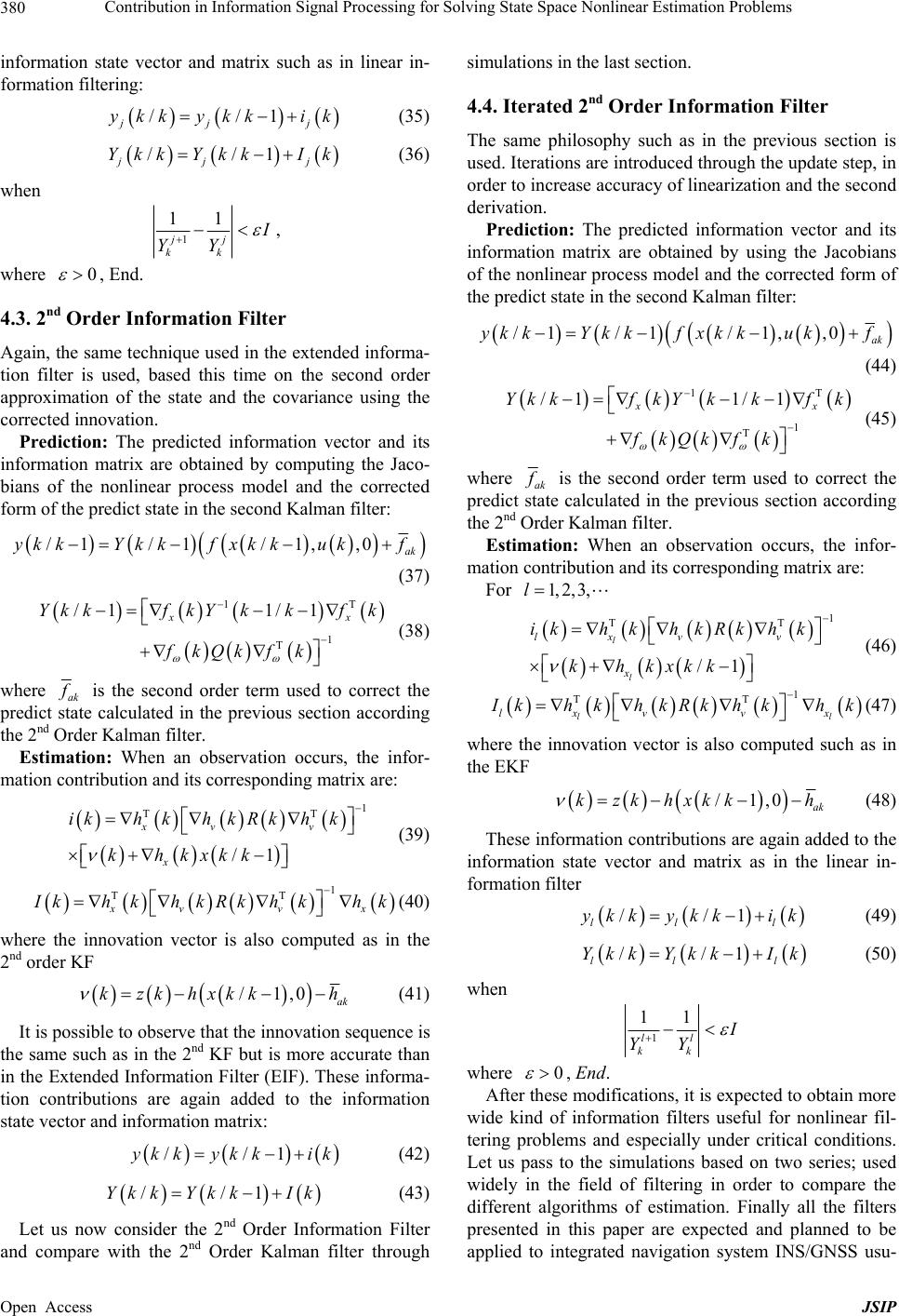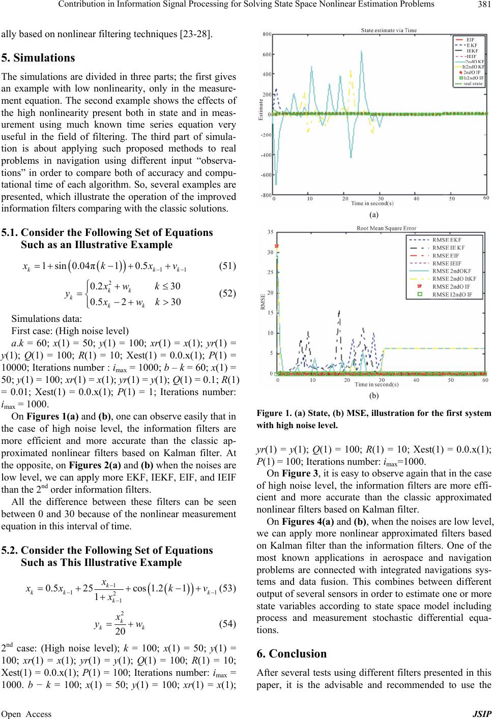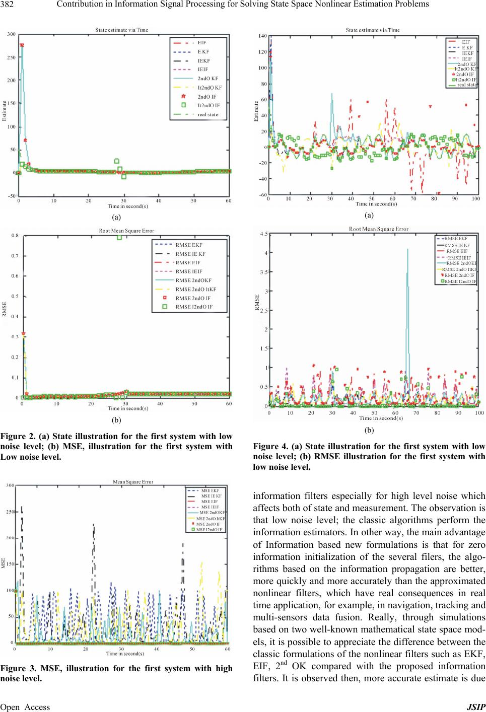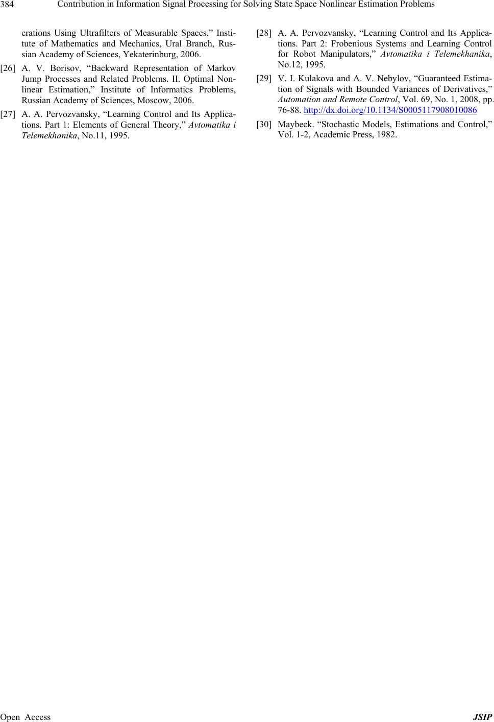
Contribution in Information Signal Processing for Solving State Space Nonlinear Estimation Problems 383
to high nonlinearity both in system and measurement
equations using new formulations of iterative extended
Kalman filter, 2nd order information filter and 2nd order
iterative information filter. Finally, original formulations
based on sigma point Kalman filters and divided differ-
ence information filters are considered to be completed
in the near future. It is expected in the future to apply
these information filters to integrated navigation system
based on combination between GNSS (GPS/GLONASS)
and Inertial navigation system (INS) using nonlinear
measurement equations in order to compare and confirm
that really the new formulations give more accuracy in
state estimation’s problems such as started in [29,30] and
improved by the novel formulation proposed in this work.
Finally, original formulations based on sigma point Kal-
man filters and divided difference information filters are
considered to be completed in the near future, with addi-
tional ways of research on adaptive and robust formula-
tions of information filters in very aggressive noise en-
vironment.
REFERENCES
[1] R. E. Kalman and R. S. Bucy “A New Approach to Lin-
ear Filtering and Prediction Problems,” Journal of Basic
Engineering, Vol. 82, No. 1, 1960, pp. 35-45.
http://dx.doi.org/10.1115/1.3662552
[2] R. E. Kalman and R. S. Bucy, “New Results in Linear
Filtering and Prediction Theory,” Journal of Basic Engi-
neering, Vol. 83, No. 1, 1961, pp. 95-108.
http://dx.doi.org/10.1115/1.3658902
[3] J. Kim, “Autonomous Navigation for Airborne Applica-
tions,” Department of Aerospace, Mechanical and Mecha-
tronic Engineering, The University of Sydney, Sydney,
2004.
[4] A. V. Nebylov, “Ensuring Control Accuracy,” Springer
Verlag, Heidelberg, 2004. 244 p.
http://dx.doi.org/10.1007/b97716
[5] T. Lefebvre, et al. “Kalman Filters for Nonlinear Sys-
tems,” Nonlinear Kalman Filtering, Vol. 19, 2005, pp.
51-76.
[6] S. Thrun, D. Koller, Z. Ghahramani, H. Durrant-Whyte
and Y. Ng Andrew, “Simultaneous Mapping and Local-
ization with Sparse Extended Information Filters: Theory
and Initial Results,” University of Sydney, Sydney, 2002.
[7] Y. Liu and S. Thrun, “Results for Outdoor-SLAM Using
Sparse Extended Information Filters,” Proceedings of
ICRA, 2003.
[8] M. Simandl, “Lectures Notes on State Estimation of Non-
Linear Non-Gaussian Stochastic Systems,” Department of
Cybernetics, Faculty of Applied Sciences, University of
West Bohemia, Pilsen, 2006.
[9] A. Mutambara, “Decentralised Estimation and Control for
Multisensor Systems,” CRC Press, LLC, Boca Raton,
1998.
[10] J. Manyika and H. Durrant-Whyte, “Data Fusion and Sen-
sor Management: A Decentralized Information-Theoretic
Approach,” Prentice Hall, Upper Saddle River, 1994.
[11] A. Gasparri, F. Pascucci and G. Ulivi, “A Distributed
Extended Information Filter for Self-Localization in Sen-
sor Networks,” Personal, Indoor and Mobile Radio Com-
munications, 2008.
[12] M. Walter, F. Hover and J. Leonard, “SLAM for Ship
Hull Inspection Using Exactly Sparse Extended Informa-
tion Filters,” Massachusetts Institute of Technology, 2008.
[13] G. Borisov, A. S. Ermilov, T. V. Ermilova and V. M. Suk-
hanov, “Control of the Angular Motion of a Semiactive
Bundle of Bodies Relying on the Estimates of Non-
measurable Coordinated Obtained by Kalman Filtration
Methods,” Institute of Control Sciences, Russian Acad-
emy of Sciences, Moscow, 2004.
[14] N. V. Medvedeva and G. A. Timofeeva, “Comparison of
Linear and Nonlinear Methods of Confidence Estimation
for Statistically Uncertain Systems,” Ural State Academy
of Railway Transport, Yekaterinburg, 2006.
[15] H. Benzerrouk and A. Nebylov, “Robust Integated Navi-
gation System Based on Joint Application of Linear and
Non-Linear Filters,” IEEE Aerospace Conference, Big
Sky, 2011.
[16] H. Benzerrouk and A. Nebylov, “Experimental Naviga-
tion System Based on Robust Adaptive Linear and Non-
Linear Filters,” 19th International Integrated Navigation
System Conference, Elektropribor-Saint Petersburg, 2011.
[17] H. Benzerrouk and A. Nebylov, “Robust Non-Linear Fil-
tering Applied to Integrated Navigation System INS/
GNSS under Non-Gaussian Noise Effect, Embedded Gui-
dance, Navigation and Control in Aerospace (EGNCA),”
2012.
[18] T. Vercauteren and X. Wang, “Decentralized Sigma-Point
Information Filters for Target Tracking in Collaborative
Sensor Networks,” IEEE Transactions on Signal Proc-
essing, 2005. http://dx.doi.org/10.1109/TSP.2005.851106
[19] G. J. Bierman, “Square-Root Information Filtering and
Smoothing for Precision Orbit Determination,” Factor-
ized Estimation Applications, Inc., Canoga Park, 1980.
[20] M. V. Kulikova and I. V. Semoushin, “Score Evaluation
within the Extended Square-Root Information Filter,” In:
V. N. Alexandrov, et al., Eds., Springer-Verlag, Berlin,
2006, pp. 473-481.
[21] G. J. Bierman, “The Treatment of Bias in the Square-Root
Information Filter/Smoother,” Journal of Optimization
Theory and Applications, Vol. 16, No. 1-2, 1975, pp. 165-
178. http://dx.doi.org/10.1007/BF00935630
[22] C. Lanquillon, “Evaluating Performance Indicators for
Adaptive Information Filtering,” Daimler Chrysler Re-
search and Technology, Germany.
[23] V. Yu. Tertychnyi-Dauri, “Adaptive Optimal Nonlinear
Filtering and Some Adjacent Questions,” State Institute
of Fine Mechanics and Optics, St. Petersburg, 2000.
[24] O. M. Kurkin, “Guaranteed Estimation Algorithms for
Prediction and Interpolation of Random Processes,” Sci-
entic Research Institute of Radio Engineering, Moscow,
1999.
[25] A. G. Chentsov, “Construction of Limiting Process Op-
Open Access JSIP

Contribution in Information Signal Processing for Solving State Space Nonlinear Estimation Problems
Open Access JSIP
384
erations Using Ultrafilters of Measurable Spaces,” Insti-
tute of Mathematics and Mechanics, Ural Branch, Rus-
sian Academy of Sciences, Yekaterinburg, 2006.
[26] A. V. Borisov, “Backward Representation of Markov
Jump Processes and Related Problems. II. Optimal Non-
linear Estimation,” Institute of Informatics Problems,
Russian Academy of Sciences, Moscow, 2006.
[27] A. A. Pervozvansky, “Learning Control and Its Applica-
tions. Part 1: Elements of General Theory,” Avtomatika i
Telemekhanika, No.11, 1995.
[28] A. A. Pervozvansky, “Learning Control and Its Applica-
tions. Part 2: Frobenious Systems and Learning Control
for Robot Manipulators,” Avtomatika i Telemekhanika,
No.12, 1995.
[29] V. I. Kulakova and A. V. Nebylov, “Guaranteed Estima-
tion of Signals with Bounded Variances of Derivatives,”
Automation and Remote Control, Vol. 69, No. 1, 2008, pp.
76-88. http://dx.doi.org/10.1134/S0005117908010086
[30] Maybeck. “Stochastic Models, Estimations and Control,”
Vol. 1-2, Academic Press, 1982.