Paper Menu >>
Journal Menu >>
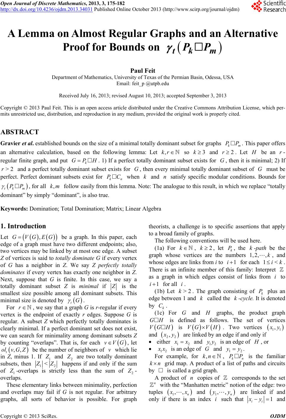 Open Journal of Discrete Mathematics, 2013, 3, 175-182 http://dx.doi.org/10.4236/ojdm.2013.34031 Published Online October 2013 (http://www.scirp.org/journal/ojdm) A Lemma on Almost Regular Graphs and an Alternative Proof for Bounds on tk m P P Paul Feit Department of Mathematics, University of Texas of the Permian Basin, Odessa, USA Email: feit_p @utpb.edu Received July 16, 2013; revised August 10, 2013; accepted September 3, 2013 Copyright © 2013 Paul Feit. This is an open access article distributed under the Creative Commons Attribution License, which per- mits unrestricted use, distribution, and reproduction in any medium, provided the original work is properly cited. ABSTRACT Gravier et al. established bounds on the size of a minimal totally dominant subset for graphs . This paper offers an alternative calculation, based on the following lemma: Let km PP ,kr so and . Let 3k2r H be an - regular finite graph, and put . 1) If a perfect totally dominant subset exists for , then it is minimal; 2) If and a perfect totally dominant subset exists for , then every minimal totally dominant subset of must be perfect. Perfect dominant subsets exist for when and satisfy specific modular conditions. Bounds for , for all follow easily from this lemma. Note: The analogue to this result, in which we replace “totally dominant” by simply “dominant”, is also true. r k GPHG >2r tk P G G k PCn kn m P,km Keywords: Domination; Total Domination; Matrix; Linear Algebra 1. Introduction Let be a graph. In this paper, each edge of a graph must have two different endpoints; also, two vertices may be linked by at most one edge. A subset Z of vertices is said to totally dominate G if every vertex of G has a neighbor in Z. We say Z perfectly totally dominates if every vertex has exactly one neighbor in Z. Next, suppose that G is finite. In this case, we say a totally dominant subset Z is minimal if ,GVGEG Z is the smallest size possible among all dominant subsets. This minimal size is denoted by tG . For , we say that a graph G is r-regular if every vertex is the endpoint of exactly r edges. Suppose G is regular. A subset Z which perfectly totally dominates is clearly minimal. If a perfect dominant set does not exist, we can search for minimality among dominant subsets Z by counting “overlaps”. That is, for each r vVG v, let t be the number of neighbors of which lie in Z, minus 1. If ,,G Z ol v 1 Z and 2 Z are two totally dominant subsets, then 12 < Z Z happens if and only if the sum of 1 Z -overlaps is strictly less than the sum of 2 Z - overlaps. These elementary links between minimality, perfection and overlaps may fail if G is not regular. For arbitrary theorists, a challenge is to specific assertions that apply to a broad family of graphs. The following conventions graphs, all sorts of behavior is possible. For graph will be used here. (1a) For k , 2k, let k P, the k-path be the graph whosece the numbers 2,, k, and whose edges are links from i to 1i for each <ik vertis are1, 1 . There is an infinite member of family: Inte as a graph in which edges consist of links from i 1i this rpret to for all i. b) Let >k (1 The graph consisting of plus an ed ) Fo and 2. n 1 an r G k P isge betweed k called the k-cycle. It denoted by k C. (1c H graphhe prct graph s, todu GH is deed asllows. The set of vertices fin fo H is VG VG VH. Two vertices 11 , x y and 22 , x y r aredge if and only if ei 2 e linke an d by the 1 x x and 12 yy is an edge of H , or 12 x x is an edge of G and 12 yy. For example, for ,kn , kn PP is the familiar kn grid map. A proa aths and circuits is called a grid graph. A product of n copies of duct of list of p by corresponds to the set n with the “Mahatten metric” notion of the edge: two les tup n 1,, n x x and 1,, n y y are linked if and only if index at there is anith such 1 ii xy and C opyright © 2013 SciRes. OJDM 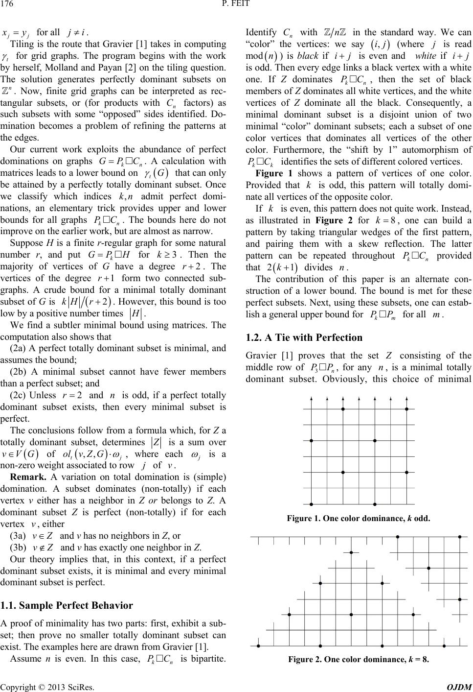 P. FEIT 176 j j x y for all ji. Tiling is the route that Gravier [1] takes in computing t for grid graphs. The program begins with the work herself, Molland and Payan [2] on the tiling question. The solution generates perfectly dominant subsets on n . Now, finite grid graphs can be interpreted as rec- ular subsets, or (for products with n C factors) as such subsets with some “opposed” sides intified. Do- mination becomes a problem of refining the patterns at the edges. Our curr by tang do nu de ent xploits the abundance of perfect work e minations on graphs kn GPC. A calculation with matrices leads to a lower tG that can only be attained by a perfectly totally dot subset. Once we classify which indices ,kn admit perfect domi- nations, an elementary trick ides upper and lower bounds for all graphs kn PC. The bounds here do not improve on the earlier wt are almost as narrow. Suppose H is a finite r-regular graph for some natural bound on prov ork, bu minan mber r, and put k GPH for 3k. Then the majority of vertices a de2r of G havegree . The vertices of the degree 1r form two conn sub- graphs. A crude bound for minimal totally dominant subset of G is ected a 2kH r. However, this bound is too low by a positives e number tim H . We find a subtler minimal bo usinundhe t subset is minimal, and bset cannot have fewer members is odd, if a perfect totally e nclusions follow from a formula which, for Z a g matrices. T co as tha do tot mputation also shows that (2a) A perfect totally dominan sumes the bound; (2b) A minimal su n a perfect subset; and (2c) Unless 2r and n minant subset exists, thn every minimal subset is perfect. The co ally dominant subset, determines Z is a sum over vVG of ,, tj olvZ G , where each j is a w j of v. Remark. A variation on total dinatin non-zero do do 1.1. Sa weight associated to ro omois (simple) d v has no neighbors in Z, or Z. rfect mple Perfect Behavior ts: first, exhibit a sub- ite. Id mination. A subset dominates (non-totally) if each vertex v either has a neighbor in Z or belongs to Z. A dominant subset Z is perfect (non-totally) if for each vertex v, either (3a) Z anv (3b) and v has exactly one neighbor invZ Our theory implies that, in this context, if a pe minant subset exists, it is minimal and every minimal dominant subset is perfect. A proof of minimality has two par set; then prove no smaller totally dominant subset can exist. The examples here are drawn from Gravier [1]. Assume n is even. In this case, kn PC is bipart entify n C with n in the stanway. We can “color” the vertices: we say ,ij (where j is read mod dard n) is black if ij is eand whit if ijven e is odhen every edgks a black vertex with a w one. If Z dominates kn PC, then the set of black members of Z dominates all white vertices, and the white vertices of Z dominate all the black. Consequently, a minimal dominant subset is a disjoint union of two minimal “color” dominant subsets; each a subset of one color vertices that dominates all vertices of the other color. Furthermore, the “shift by 1” automorphism of kk PC identifies the sets of different colored vertices. re 1 shows a pattern of vertices of one color d. T igu us e linhite . stead, F Pr as ovided that k is odd, this pattern will totally domi- nate all vertices of the opposite color. If k is even, this pattern does not quite woInrk. illtrated in Figure 2 for 8 k, one can build a pattern by taking triangular wedof the first pattern, and pairing them with a skew reflection. The latter pattern can be repeated throughout kn PC provided that ges 21k divides n. Thbution of his pae contritper is a set n alternate con- struction of a lower bound. The bound is met for these perfect subsets. Next, using these subsets, one can estab- lish a general upper bound for km PP for all m. 1.2. A Tie with Perfection Gravier [1] proves that the Z consisting of the middle row of 3n PP, for any n,s a minimal totally dominant subset. Obviously, this choice of minimal i Figure 1. Once, k odd.e color dominan Figure 2. Once, k = 8. e color dominan Copyright © 2013 SciRes. OJDM  P. FEIT 177 For each integer 1jk , put subset pro blocks, duces many overlaps. By rotating 33 we can produce other minimal dominant seth fewer overlaps, as in Figure 3. Furthermore, if n is a multiple of 4, there is a variation which is a perfect total domination of 3n PC, as in Figure 4. The flexibility in the number of s which are dominated by more than one member of ts wi vertice Z reflects the presence of vertices of two degrees, namely 3 and 4. In this example, the size of a minimal, imperfect to 1.3. Weights ts of theorems based on series. tally dominant subset “ties” the size of a perfect totally dominant set. Can a minimal subset be smaller than a perfect one? We prove that a tie is rare, and that beating is impossible. We have two se Definition 1 Let r be a real number. Let r i a be the set of infinite sequences of real numbers 0i such that 12 1, . iii iaraa Clearly, r 1 ii . is a real vector space, and the fu real, let ibe the unique member of nction ,aaa is a linear isomorphism from it onto For 01 2 r ,ir r sch that and ,1 1r . Observe ,2rr . In that th u e o ,0 0r g section, we defpeninip function ned the overla ,, tv G Z for totally dominant subsets Z of a graph G. or G a graph and Z a dominant (but possibly not totally) subset, and vVG, let ,,olv GZ be ,, t olvGZ if vZ an,G ZZ ol In addition, f d , t ol v 1 if v . , GPH fh H vVefine the row of v to be the first of v. Lemma 2 Lt For >3k G, d coordinate k row or som e grap and v e such that and ,rk 2r3k. Figure 3. Two ways to totally dominate 3n P P. Figure 4. Perfect domination in 34m P C. 1 ,j rk 1 1,1 1, . j kj rk j rj For each 1jk , 0 (4a) j , and (4b) 0 j if and only if is odd and is fer to 2r, k j even. We re1,, k as the weight system for para- mition 3 Let eters ,rk. Defin ,rk such that and 2r 3. Let 1,, k k weight system,rk. let 1, be the for Also, , k be the weight system for parame 1,rk ters . D efine 1 2 22,12 ,12 , . 2,1 k rk kr kr k rk rrk Suppose is an regular graph, and put r-nH H and k GPH . Define two functions on Z VG: , ,ZolvZG row row score score, , tt v vVG tv vVG Zo lvZGv Theorem 4 Assume the hypothesis and construction of Lemma 2 and Definition 3. Let H be a finite graph, and put nH and k GPH . (A) If Z VG is totally dominant, then scoretZ , . 2, 1 Znrk rrk (B) If Z VG is dominant, then scoreZ 1, . 31,1 Znr krrk A trivial consequence of this theorem and the pre- ce ume the hypothesis of Theorem 4. ding lemma is: Corollary 5 Ass (A) Suppose 3r. If 12 , Z Z are totally dominant subsets of G, then 121 2 < score<score . tt Z ZZZ (B) If 12 , Z Z are do minant su bsets of then G, 1 2 score<score . 12 < Z ZZ Z 2. Modeled with Matrices linear algebra model. Our results are based on a simple For convenience, (5) For k , let Ind1, ,kk. Notation et k 6. L . We identify the real vector space k with lengolumn vectors. We use trans- th k c Copyright © 2013 SciRes. OJDM  P. FEIT 178 pose notation to write these horizontally: z 1 T 1 (,,) for . k k zz z For each , let 1iki k nal be the projection function from each v ,,zz to its i-coordinate i z. Also define a linear fk k ector 1 unctio 1 π. i i s um zz We denote the zero vector by d let H be a finite, ˆ 0. , aIn what follows, let ,krn r-regular graph. Put G. For k PH Z VG, de cfine the rowount vector z for Z to be in in the th u z which i z is the number of members T 1,, k z of Z row. Obviosly, i- s um zZ. Now sup ose p Z VG totally dominates, and let ,,z z beount vector. Let 1ik 1k z its row c . ,, t lvZ G over all v in the i-th r The sum of oow, plus H , equals rz12 11 1 ,for 1, ,for 11,and ,for . ii i kk z i zrz zik zrz ik (6) In particular, lly dominates, then each of these ex- pr (7a) If Z tota essions must be H , and (7b) If Z perfectllly domy totainates, then each of these expressions must equal H . If we replace totallymi donation with simple domi- na ivate r next definition. t be a na tion, the analogous assertions hold after the r terms in (6) are changed to 1r. These remarks motou Definition 7 Let r be a real number and lek tural number >1. Define ,Lrk to be the kk matrix such that , if , ,Ind, ,1ifis1or1 0otherwise. ij rij ijkLrkij , Note that ,Lrk hese pa is symmetric. Also, for trameters, define , M rk to be the Note that the case is covered in both parts of this conditional definition. atrix kk matrix such that ,Ind, ij k , ,, 1if , ,,,1if . ij ri rkji j Mrk rjrkij i is essentially 1 ,rkL . 3. Relevant Sequences convexity for functions of a ij As we shall see, the m , M rk There is a discrete analogy to single real variable. We recall some basics. Definition 8 Let 0 i ai be a sequence of real num- bers, starting at index We say that the sequence is convex if 0. 11 , . iiii iaaaa We say a the sequence is strictly convex if 11 > iiii aaa for each i. 0 i aLemma 9 Let i be a convex sequence. For ,vu , 0 . uvuv aaaa Moreover, 0uvu v aaaa ch that if and only if there is a number t su 1 , . ii uvata Indi Proof. ge We may interchange u and v without loss of nerality. Hence, assume uv. For each i , put 1iii baa . Then 1 i bi weakly incr se- is a easing quence. Then 00 0 111 0 11 01 11 01 1 u v uv uv iii iii vv uv u vuii ii vv uvuvuv ji ji v uvuvuvii i aaaa bbb aaaabb aaaabb aaaab b uv Obse aa (8) rve that 21 ii uv vi1uv 0. For eac fo h index i in the last sum, the term has the rmat p q bb where >pq. Therefore 00. uv aa a u v a Now s00 uv uv aaaa . ) must be 0. Wh Then every term uppose in the final sum of (8en 1i, we get 10 uv bb . Since i b is an increasing ence, it 1i bb sequ follows that foevery index iuv. □ We focus sequences ,r finition 1. r the i on of De 0 Let r be a real number. Then Trivial. □ Th Proof. e first remark is that the sign ceparated from the magnitude. Lemma 1 an be s 1 , 1,, . i iriri Copyright © 2013 SciRes. OJDM  P. FEIT 179 Many of the positive sequences ,ri are convex. Lemma 11 Each member of 2 is a linear se- qu Trivial. □ ence. Proof. Lemma 12 Let >2r, and let i br such that 1 b0 0b. If 1 bthen >0 , i basing and more, 1ii bb can occur only if 1i. is incre strictly convex. Further Proof. For , we can rewrite the relation 2i s 12ii rb b a i b (9a) 11 12iiii b bb 2bbrbb b 2bi 111iiiii the two identities to induct on br, and 2 the double hy- po 2 . □ Corollary 13 Let and su (9b) . Use thesis that both >>0 anbb 111 d >>0 iiiii i bbbb rkch that 2. Then r ,rk of. This 0 . an easy conse Pro quence mma and Le Fo is of this le mma 10. □ The next two propositions play roles in our analysis. Lemma 14 Let r be a real number other than 2. r 1k, 1 ,1, 1 , 2. i rk rk ri r (10) Proof. In what follows, a sum from any integer to k m v 1 is defined to be 0. For this proof, we abbreiate m k For for ,rk . each 0k, define 0 , . ki k s ri Then for i Define a new sequence by 2k, 2 12 10 12 011 2 1 1 . k ki kk jj kk sri rj j rs s 1 2 ii tsr . Replace 1 2 ii str into the previous relation to get k Hence, 1 2, . kk ktrtt i t belongs to r. Now 00 11 11 22 11 . 22 tsrr r tsrr 2 , In the vector space 111 1 , 1,0,1. 22 22 rr rr rr The sequences i t and 11 1 22 ii i rr both belong to r th , and agree on the first two indices. He sequence. This gives the equality of (10). □ Lemma 15 Let ence, they are e sam r be a real number, and let ,jk such that kjn . The ,1,, 2 ,1,1 . rkr jrkj rjrk j Proof. We write i for ,ri in this a If kj r gu men t. , then 22kj r , 111kj recu defin , and the f ition. result ollows from a proo 1 .j from the rsive The remaining cases follow f is by in- duction on j. The inductive hypothesis is 1kj , 21 kj kjjk For 1j , this follows from the fact that 11 and 00 . Assume j for which the inductive hy true. Let pothesis is k so >1kj . Then 21 11jkj jkj rj j 1 11 11 211 1 . k j jkj jrk jkjjk j jkjjk j k 11 1 kjj kj rj jkj 1 □ 4. The Inverse Matrices We can now prove Lemma 16 Let k and . The matric pr duct ro- ,,Lrk Mrk is ,1rk times the iden- tity matrix. ent, let Proof. For this argum ,LLrk and , M Mrk and, for each i 0, let ,iri . Le ,Induvthe lemma by comparing the v en and k. We prove t ,utry of LM 1k times the u,v entry of the identhere a t of cases. ity matrix. T lo Case re a 1u . For any vk Ind , Copyright © 2013 SciRes. OJDM 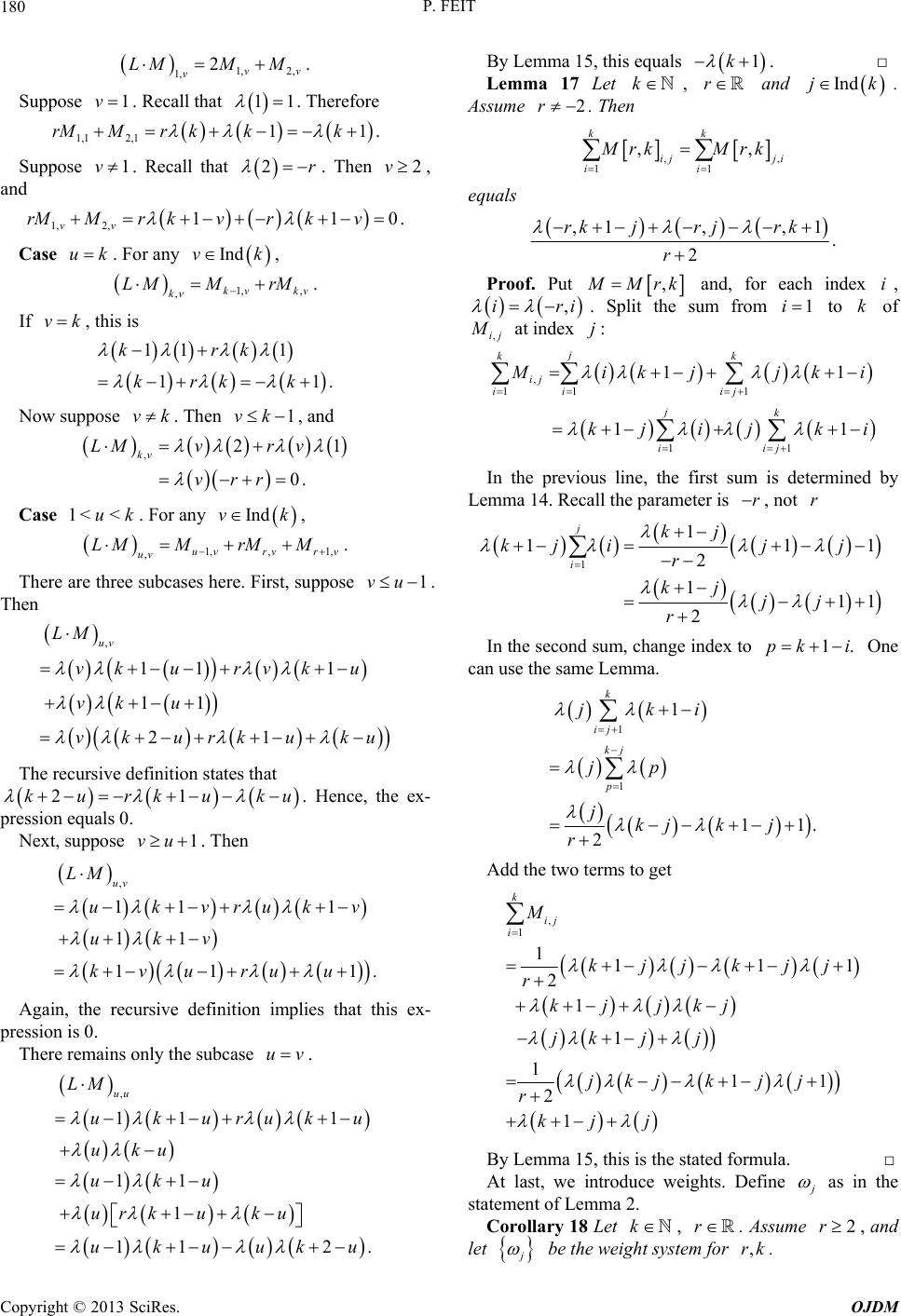 P. FEIT 180 1,2, . vv v LM M Suppose 1. Recall that 11 . Therefore 1, 2M v 1,1 11Mrkkk . 2,1 Suppose1. Recall that rM v 2r . Then and . Case . For any , this is 2v, 1, 110 vv rMMrkvkv 2, r uk Indvk, , . v kv L rM 1, ,k kv M M If vk 11 1 krk rk k 1k 1. Now suppose . Then , and vk 1vk ,21 0 . kv vr v vrr Case . For any There are three subcases here. First, suppos LM 1< <uk Indvk, LM MM 1,, 1, , . uvrv rv uv rM e 1vu . Then The recursive definition states that Hence, thex- Next, suppose . Then 1 . Again, the recursive definition implies that this ex- pression is 0. There remains only the subcase . By Lemma 15, this equals □ Lemma 17 Let L , 11 1 21 uv M vk urvk vk urkuku 11vk u u 21kurkuku . pression equals 0. e 1vu 11 1 LM uk vru kv vuu u , 1 1 uv kv u 11kr uv. , 1 11 2 uu LM ku ur kuku ukuuku 111 uk uruku u 11uk u 1k . k , r and In djk. Assume 2r . Then ,, 11 ,, kk ij ji ii M rkMrk equals ,1, ,1 . 2 rkjr jrk r Proof. Put , M Mrk , iand, for each index ithe s, ,ij ir . Split um from to 1ik of M at index j: , 1 1 11 11 11 j kk ij i ij jk iij 1i M ikjjk i kj ijk i In the previofirst sum is determined by all the parameter is us line, the Lemma 14. Rec r , n r ot 1 1 11 2 111 1 2 i kj kj ijj r kjjj r j In the second sum, change index to One ca 1.pk i n use the same Lemma. 1 1 1 k jki 11. ij kj p jp jkjk j 2r Add the two terms to get 1jk j , 1 1111 2 1 1 11 2 1 k ij i M kjjkj r kj jkj jk jj kjj r kj j j By Lemma 15, this is the stated formula. □ At last, we introduce weights. Define j as in the statement of Lemma 2. Corolla ry 18 Let k , . Assume and let r2r, j be the we ight system for ,rk. Copyright © 2013 SciRes. OJDM 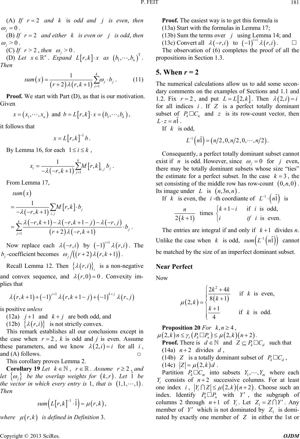 P. FEIT 181 (A) If and is odd and is even, then 2r kj 0 j . (B) If nd eith is even is odd, th e n 2r aer k or j >0 j . (C) If >2r, then >0 j . (D) Let xn . Expand ,Lrkx as Then T 1,,bb. n 1 1 . 2,1 k j j j s um xb rrk (11) Proof. We start with Part (D), as that is our motivation. Given 11 ,, and ,,, , nk x xx bLrkxbb it f ollows that 1 , . x Lrkb Bemm1 ik , y La 16, for each , 1j 1k , . ,1 ij ij x Mrk b rk ma 17 From Lem, , 1 1, ,1 . 2,1 j ij ,1 ,1 , k j j m x Mrk b rk b rrk each su rkrkjr j Now replace ,ri by. The 1 1, iri j b-coefficient becomes 2,1rrk . j Recall Lemma 12. Then is a non-negative an ,i ri d convex sequence, and ,0 0r . Convexity im- plies that k is (12a) and are both odd, and (12b) trictly convex. This lishes all our conclusions excep in the case when k is odd and j is even. Assume these parameand we know for all a nd (A) follow This corollary proves Lemma 2. 1 ,1 1,11, j rkrkjr j j positive unless 1j , kj is not s ri remark estabt 2r, ters, s. 2,ii i, □ Corolla ry 19 Let k,r . A, and ssume let 2r j be the overla in which every p w eeights f try is 1, or be n Th ,kr that is . Let ˆ 1 1,1, the vector ,1 . en 1 , , ˆ 1 , s umLrk r k where is defined in Definition 3. Proof. The easiest way is to get this formula is (13a) Start with the formulas in Lemma 17; s over using Lemma 14; and onv ,rk (13b) Sum the termj (13c) Cert all ,ri to 1 1, iri roof o . servationf all th pr dae examles ofnd 1. Fi e The ob of (6) completes the p opositions in Section 1.3. 5. When r = 2 Th s to add some secon-e numerical calculations allow u ry comments on thp Sections a1 and 1.2. x2r , and put 2,LL k. Then 2,ii for all indices i. If Z is a perfect totallyt subset of PC and z is its row-count v dominan ector, then kn ˆ 1Lz n . is odd, If k ˆ 12,0, 2,0, , 2n nnn 1 .L cannot ex Consequently, a perfect totally dominant subset ist if n is odd. However, since 0 j for j even dominabsets who , th s th ere may be totallynt sue size “ties” e estimate for a perfect subset. In the case 3k , the set consisting of the middle row has row-count 0, ,0n. Its image under L is ,n. -th coordia ,3nn If k is even, the n ite of 1 ˆ 1Ln is 1ifis odd, times is even. 21 ki i n iifi k The entre integral i if 1k di. Unlike the case hen k is odd, 1ˆ 1 ries af and onlyvides n w s um Ln cannot be matched by the size of an imperfect dominant subset. Near Perfect Now 2 24 ifis even, 81 2, 1ifis odd. 4 kk k k kkk Prosition 20 Fo ,4kn, op r 2, 2 tk n knPPn 2, k . Proof. There is d and kd Z PC suchat (14a) th 2n divides d, (14b) Z is a totally dominant subset okd C, Pf (14c) 2, Z kd Partition km PC in subsets re each . to whe 1,, m YY i Y consists of 2n successive columns. For at least ndex one ii, 2, i YZ k 2n . Ch , the su kn PP with Y rough 1n oose such an bgraph of ns 2 index. Identify colum th of i Y. Let 1 Z ZY . Any er ofmemb Y which is not dominated by 1 Z is domi- ed by enatxactly one member of Z in either the 1st or Copyright © 2013 SciRes. OJDM 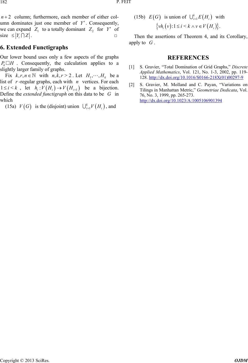 P. FEIT Copyright © 2013 SciRes. OJDM 182 column; furthermore, each member of either col- inates just one member of . Consequently, n expand (15b) EG is union of 1 k ii EH with : 1< . i vhvikvVH 2n umn dom we ca Y 1 Z Y to a totally dominant 2 Z for of size i YZ 6. Our lo P sli i the asser Theoremd its Coro o [1] ravier,d Graphs,” D lied Ma 121, No. 1-3, 2002, pp. 119- 128. http://dx.doi.org/10.1016/S0166-218X(01)00297-9 . □ igraph wer bouuses only a few as the hs ntly, alculaa arger rhs. nd e pect tion of grap k Thentions of 4, anllary, apply t G. REFERENCES Extended Functs s k ghtly lfamily of gap H. Consequthe capplies to S. G “Total Domination of Griiscrete App thematics, Vol. Fix k n with ,,>2nkr . Let 1 ,,r,, H H vertices. For eac be a h he (dnio lis 1 De t of r-regular graphs, eac :h ed t h with n be <ik , l 1ii VH VH a bijection. fine the extend nctigraph on this data to be G in which (15a) VG isisjoint) un 1 k ii VH , and [2] S. Gravier, M. Molland and C. Payan, “Variations on //d oi.org/10.1023/A:1005106901394 et i fuTilings in Manhattan Metric,” Geometriae Dedicata, Vol. 76, No. 3, 1999, pp. 265-273. http: x.d |