Open Journal of Applied Sciences, 2013, 3, 381-392
http://dx.doi.org/10.4236/ojapps.2013.36048 Published Online October 2013 (http://www.scirp.org/journal/ojapps)
The Effect of Hygroscopic Growth on Continental Aerosols
Bello Idrith Tijjani1, Aliyu Aliyu2, Fatima Shuaibu3
1Department of Physics, Bayero University, Kano, Nigeria
2Department of Science Laboratory Technology, School of Technology, Kano State Polytechnic, Kano, Nigeria
3Girl’s Science and Technical College, Kano, Nigeria
Received July 11, 2013; revised August 30, 2013; accepted September 12, 2013
Copyright © 2013 Bello Idrith Tijjani et al. This is an open access article distributed under the Creative Commons Attribution Li-
cense, which permits unrestricted use, distribution, and reproduction in any medium, provided the original work is properly cited.
ABSTRACT
In this paper, the authors investigated some microphysical and optical properties of continental clean aerosols from
OPAC to determine the effect of hygroscopic growth at the spectral range of 0.25 μm to 2.5 μm and eight relative hu-
midities (RHs) (0%, 50%, 70%, 80%, 90%, 95%, 98% and 99%). The microphysical properties extracted were radii,
volume mix ratio, number mix ratio and mass mix ratio as a function of RH while the optical properties are scattering
and absorption coefficients and asymmetric parameters. Using the microphysical properties, growth factors of the mix-
tures were determined while using optical properties the enhancement parameters were determined and then parameter-
ized using some models. We observed that the data fitted the models very well. The angstrom coefficients show that the
mixture has bimodal type of distribution with the dominance of fine mode particles.
Keywords: Microphysical Properties; Optical Properties; Hygroscopic Growth; Parametrization; Enhancement
Parameters; Angstrom Coefficients
1. Introduction
Aerosol in the atmosphere is comprised of numerous and
diverse components originating from both natural and an-
thropogenic activities.
An important factor affecting the role aerosols play in
climate change is their hygroscopicity and is currently
modeled in global climate models (GCMs), mostly to
better predict the scattering properties and size distribu-
tion under varying humidity conditions [1]. The swelling
of aerosols due to water vapor uptake will enhance their
ability to scatter radiation. Numerous studies have inves-
tigated the relationship between aerosol scattering and
relative humidity RH in terms of the hygroscopic growth
factor gf(RH) using humidified nephelometers. These
have been used for airborne or ground-based determina-
tion of the growth factor considering a “dry” RH over the
range from 20% - 40% and a ‘‘wet’’ RH up to 90% [2-5].
The characterization of particle hygroscopicity has
primary importance for climate monitoring and predic-
tion. Model studies have demonstrated that relative hu-
midity (RH) has a critical influence on aerosol climate
forcing. Hygroscopic properties of aerosols influence
particle size distribution and refractive index and hence
their radiative effects. Aerosol particles tend to grow at
large relative humidity values as a result of their hygro-
scopicity.
Some aerosol particles, such as ammonium sulphate
(NH4)2SO4, sea salt and ammonium nitrate NH4NO3 are
hygroscopic. Changes in relative humidity modify their
size distribution and refractive index and hence the opti-
cal properties of the aerosol, including the scattering co-
efficient [6-9]. Jeong et al. [10] demonstrated an expo-
nential dependence of the aerosol optical thickness on
relative humidity. A strong correlation of spectral aerosol
optical thickness with precipitable water, especially for
continental air masses, was shown by Rapti [11].
Water-soluble organic carbon (WSOC) species are
emitted as primary particles, especially during biomass
combustion, and produced as a result of reactions in the
gas and aqueous phases [12-18]. Moreover, WSOC has
been suggested as a marker for secondary organic aerosol
(SOA) in the absence of biomass burning (e.g., Docherty
et al. [19]).
In a study of aged continental aerosols, Swietlicki et al.
[7] observed 2 modes, a less hygroscopic mode with a
gf(RH) of 1.12 and a more hygroscopic mode with a
gf(RH) between 1.44 and 1.65. They postulated that the
hygroscopic growth could be attributed entirely to the
inorganic content of the aerosol: sulfate, nitrate and am-
monium ions. Particle hygroscopicity may vary as a fun-
C
opyright © 2013 SciRes. OJAppS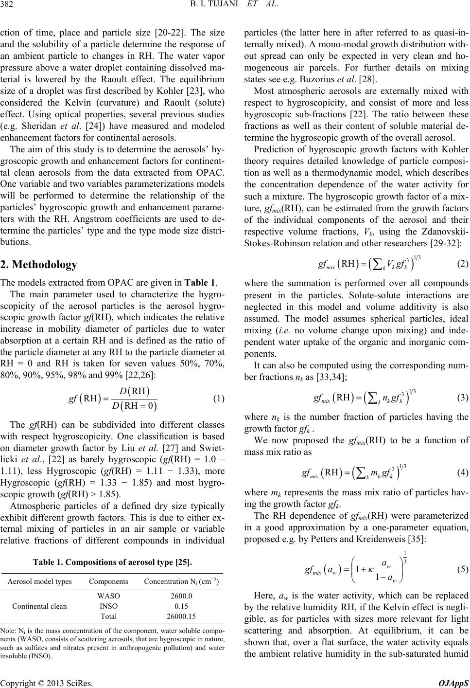

B. I. TIJJANI ET AL. 382
ction of time, place and particle size [20-22]. The size
and the solubility of a particle determine the response of
an ambient particle to changes in RH. The water vapor
pressure above a water droplet containing dissolved ma-
terial is lowered by the Raoult effect. The equilibrium
size of a droplet was first described by Kohler [23], who
considered the Kelvin (curvature) and Raoult (solute)
effect. Using optical properties, several previous studies
(e.g. Sheridan et al. [24]) have measured and modeled
enhancement factors for continental aerosols.
The aim of this study is to determine the aerosols’ hy-
groscopic growth and enhancement factors for continent-
tal clean aerosols from the data extracted from OPAC.
One variable and two variables parameterizations models
will be performed to determine the relationship of the
particles’ hygroscopic growth and enhancement parame-
ters with the RH. Angstrom coefficients are used to de-
termine the particles’ type and the type mode size distri-
butions.
2. Methodology
The models extracted from OPAC are given in Table 1.
The main parameter used to characterize the hygro-
scopicity of the aerosol particles is the aerosol hygro-
scopic growth factor gf(RH), which indicates the relative
increase in mobility diameter of particles due to water
absorption at a certain RH and is defined as the ratio of
the particle diameter at any RH to the particle diameter at
RH = 0 and RH is taken for seven values 50%, 70%,
80%, 90%, 95%, 98% and 99% [22,26]:
 

RH
RH RH 0
D
gf D  (1)
The gf(RH) can be subdivided into different classes
with respect hygroscopicity. One classification is based
on diameter growth factor by Liu et al. [27] and Swiet-
licki et al., [22] as barely hygroscopic (gf(RH) = 1.0 –
1.11), less Hygroscopic (gf(RH) = 1.11 − 1.33), more
Hygroscopic (gf(RH) = 1.33 − 1.85) and most hygro-
scopic growth (gf(RH) > 1.85).
Atmospheric particles of a defined dry size typically
exhibit different growth factors. This is due to either ex-
ternal mixing of particles in an air sample or variable
relative fractions of different compounds in individual
Table 1. Compositions of aerosol type [25].
Aerosol model types Components Concentration Ni (cm−3)
Continental clean
WASO
INSO
Total
2600.0
0.15
26000.15
Note: Ni is the mass concentration of the component, water soluble compo-
nents (WASO, consists of scattering aerosols, that are hygroscopic in nature,
such as sulfates and nitrates present in anthropogenic pollution) and water
insoluble (INSO).
particles (the latter here in after referred to as quasi-in-
ternally mixed). A mono-modal growth distribution with-
out spread can only be expected in very clean and ho-
mogeneous air parcels. For further details on mixing
states see e.g. Buzorius et al. [28].
Most atmospheric aerosols are externally mixed with
respect to hygroscopicity, and consist of more and less
hygroscopic sub-fractions [22]. The ratio between these
fractions as well as their content of soluble material de-
termine the hygroscopic growth of the overall aerosol.
Prediction of hygroscopic growth factors with Kohler
theory requires detailed knowledge of particle composi-
tion as well as a thermodynamic model, which describes
the concentration dependence of the water activity for
such a mixture. The hygroscopic growth factor of a mix-
ture, gfmix(RH), can be estimated from the growth factors
of the individual components of the aerosol and their
respective volume fractions, Vk, using the Zdanovskii-
Stokes-Robinson relation and other researchers [29-32]:


13
3
RH
mixk k
k
gfV gf (2)
where the summation is performed over all compounds
present in the particles. Solute-solute interactions are
neglected in this model and volume additivity is also
assumed. The model assumes spherical particles, ideal
mixing (i.e. no volume change upon mixing) and inde-
pendent water uptake of the organic and inorganic com-
ponents.
It can also be computed using the corresponding num-
ber fractions nk as [33,34];


13
3
RH
mixk k
k
gfn gf (3)
where nk is the number fraction of particles having the
growth factor gfk .
We now proposed the gfmix(RH) to be a function of
mass mix ratio as


13
3
RH
mixk k
k
gfm gf (4)
where mk represents the mass mix ratio of particles hav-
ing the growth factor gfk.
The RH dependence of gfmix(RH) were parameterized
in a good approximation by a one-parameter equation,
proposed e.g. by Petters and Kreidenweis [35]:

1
3
11
w
mix w
w
a
gf aa






(5)
Here, aw is the water activity, which can be replaced
by the relative humidity RH, if the Kelvin effect is negli-
gible, as for particles with sizes more relevant for light
scattering and absorption. At equilibrium, it can be
shown that, over a flat surface, the water activity equals
the ambient relative humidity in the sub-saturated humid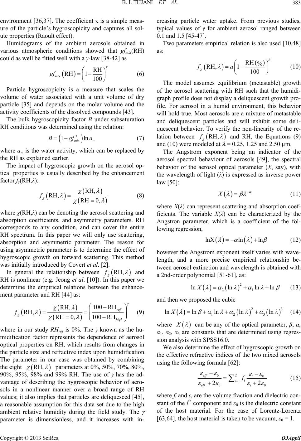

B. I. TIJJANI ET AL. 383
environment [36,37]. The coefficient κ is a simple meas-
ure of the particle’s hygroscopicity and captures all sol-
ute properties (Raoult effect).
Humidograms of the ambient aerosols obtained in
various atmospheric conditions showed that gfmix(RH)
could as well be fitted well with a γ-law [38-42] as

RH
RH1 100
mix
gf






3
1ln
mix w
Bgfa
(6)
Particle hygroscopicity is a measure that scales the
volume of water associated with a unit volume of dry
particle [35] and depends on the molar volume and the
activity coefficients of the dissolved compounds [43].
The bulk hygroscopicity factor B under subsaturation
RH conditions was determined using the relation:
(7)
where aw is the water activity, which can be replaced by
the RH as explained earlier.
The impact of hygroscopic growth on the aerosol op-
tical properties is usually described by the enhancement
factor fχ(RH,λ):


RH,
RH, RH 0, f





 (8)
where χ(RH,λ) can be denoting the aerosol scattering and
absorption coefficients, and asymmetry parameters. RH
corresponds to any condition, and can cover the entire
RH spectrum. In this paper we will only use scattering,
absorption and asymmetric parameter. The reason for
using asymmetric parameter is to determine the effect of
hygroscopic growth on forward scattering. This method
was initially introduced by Covert et al. [2].
In general the relationship between

RH,f



and
RH is nonlinear (e.g. Jeong et al. [10]). In this paper we
determine the empirical relations between the enhance-
ment parameter and RH [44] as:


100 RH RH,
RH, ref fRH 0,100 RHhigh










 

(9)
where in our study RHref is 0%. The  known as the hu-
midification factor represents the dependence of aerosol
optical properties on RH, which results from changes in
the particle size and refractive index upon humidification.
The parameter in our case was obtained by combining
the eight

RH,

 parameters at 0%, 50%, 70%, 80%,
90%, 95%, 98% and 99% RH. The use of  has the ad-
vantage of describing the hygroscopic behavior of aero-
sols in a nonlinear manner over a broad range of RH
values; it also implies that particles are deliquesced [45],
a reasonable assumption for this data set due to the high
ambient relative humidity during the field study. The 
parameter is dimensionless, and it increases with in-
creasing particle water uptake. From previous studies,
typical values of γ for ambient aerosol ranged between
0.1 and 1.5 [45-47].
Two parameters empirical relation is also used [10,48]
as:

 RH %
1100
b
fa 




RH,

(10)
The model assumes equilibrium (metastable) growth
of the aerosol scattering with RH such that the humidi-
graph profile does not display a deliquescent growth pro-
file. For aerosol in a humid environment, this behavior
will hold true. Most aerosols are a mixture of metastable
and deliquescent particles and will exhibit some deli-
quescent behavior. To verify the non-linearity of the re-
lation between


RH,f


and RH, the Equations (9)
and (10) were modeled at  = 0.25, 1.25 and 2.50 µm.
The Angstrom exponent being an indicator of the
aerosol spectral behaviour of aerosols [49], the spectral
behavior of the aerosol optical parameter (X, say), with
the wavelength of light (λ) is expressed as inverse power
law [50]:


X




 (11)
where X(λ) can represent scattering and absorption coef-
ficients. The variable X(λ) can be characterized by the
Angstron parameter, which is a coefficient of the fol-
lowing regression,


lnXln ln

   (12)
however the Angstrom exponent itself varies with wave-
length, and a more precise empirical relationship be-
tween aerosol extinction and wavelength is obtained with
a 2nd-order polynomial [51-61], as:
 
2
21
lnlnln lnX



 (13)
and then we proposed the cubic
 
23
12 3
lnln lnlnlnX

    (14)
where


X

can be any of the optical parameter, β, α,
α1, α2, α3 are constants that are determined using regres-
sion analysis with SPSS16.0.
We also determine the effect of hygroscopic growth on
the effective refractive indices of the two mixed aerosols
using the following formula [62]:
2
00
1
00
22
eff i
i
i
eff i
f









 (15)
where fi and εi are the volume fraction and dielectric con-
stant of the ith component and ε0 is the dielectric constant
of the host material. For the case of Lorentz-Lorentz
[63,64], the host material is taken to be vacuum, ε0 = 1.

B. I. TIJJANI ET AL. 384
3. Results and Observations
Figure 1 is the plot from the data of Table 2, and it
shows non-linear relation gfmix with RH, (a steep curve)
with deliquescence observed at relative humidities as
from 90% to 99% RH.
The results of the parameterizations by one and two
parameters of Equations (5) and (6) are:
C = 1.433571, k = 0.012412, R2 = 0.8731
from Equation (5)
2
0.069589, R0.9962   from Equation (6)
The fitted curve can be represented by one and two
empirical parameters fit of the form of Equations (5) and
(6), though Equation (6) has higher coefficient of deter-
mination.
Figure 2 is a plot from the data of Table 2, and shows
non-linear relation B with RH, (a steep curve) with deli-
quescence observed at relative humidities as from 90% to
99% RH.
Figure 3 is a plot from the data of Table 3, and it
shows an increase in particle diameter with increasing
RH and shows a steep curve with deliquescence observed
at relative humidities as from 90% to 99% RH.
The results of the parameterizations by a one and two
parameters of Equations (5) and (6) are:
50 55 60 65 70 75 80 85 90 95100
1.00
1.05
1.10
1.15
1.20
1.25
1.30
1.35
1.40
gf
mix
(RH)
Relative Humidity(%)
Figure 1. A graph of growth factor of the mixture using
number mix ratio (Equation (3)) against RH.
Table 2. The growth factor of the aerosols using number
mix ratio (Equation (3)) and bulk hygroscopicity factor
(Equation (7)).
RH(%) 50 70 80 90 95 98 99
gfmix(RH) 1.0731 1.1036 1.13011.1796 1.2346 1.30941.3606
Bulk
Hygroscopicity
factor (B)
0.1634 0.1228 0.0989 0.0676 0.0452 0.0252 0.0153
50 55 60 65 70 75 80 85 90 95100
0.00
0.02
0.04
0.06
0.08
0.10
0.12
0.14
0.16
Bulk Hygroscopicity Factor (B)
Relative Humidity(%)
Figure 2. Bulk hygroscopcity factor of the mixture using
number mix ratio (Equation (7)).
50 55606570 758085 90 95100
1.00
1.05
1.10
1.15
1.20
1.25
1.30
1.35
gf
mix
(RH)
Relative Humidity(%)
Figure 3. A graph of growth factor of the mixture using
volume mix ratio (Equation (2)).
Table 3. The growth factor of the aerosols using volume mix
ratio (Equation (2)) and bulk hygroscopicity factor (Equa-
tion (7)).
RH(%) 50 70 80 90 95 98 99
gfmix(RH) 1.05031.07721.1024 1.1526 1.2108 1.29101.3456
Bulk
Hygroscopicity
factor (B)
0.11000.08910.0758 0.0560 0.0398 0.02330.0144
2
C1.334733, k 0.012542, R0.8860 
from Equation (5)
2
0.064125, R0.9995   from Equation (6)
The fitted curve can be represented by one and two
empirical parameters fit of the form of Equations (5) and
(6), though Equation (6) has higher coefficient of deter-
mination.
Figure 4 is a plot from the data of Table 3, is almost the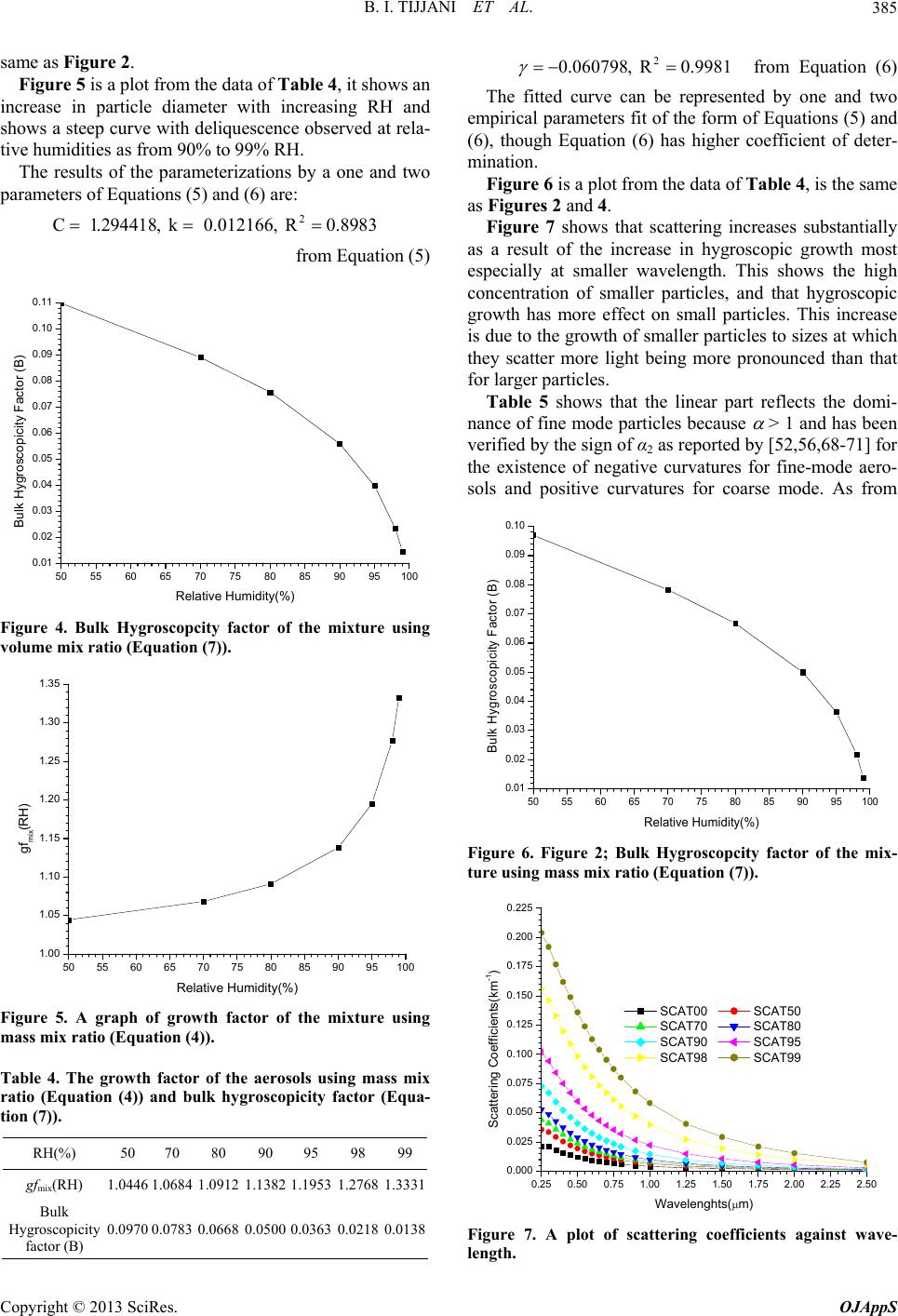

B. I. TIJJANI ET AL. 385
same as Figure 2.
Figure 5 is a plot from the data of Table 4, it shows an
increase in particle diameter with increasing RH and
shows a steep curve with deliquescence observed at rela-
tive humidities as from 90% to 99% RH.
The results of the parameterizations by a one and two
parameters of Equations (5) and (6) are:
2
C 1.294418, k 0.012166, R0.8983 
from Equation (5)
50 55 60 65 70 75 80 85 90 95100
0.01
0.02
0.03
0.04
0.05
0.06
0.07
0.08
0.09
0.10
0.11
Bulk Hygroscopicity Factor (B)
Relative Humidity(%)
Figure 4. Bulk Hygroscopcity factor of the mixture using
volume mix ratio (Equation (7)).
50 55 60 65 70 75 8085 90 95100
1.00
1.05
1.10
1.15
1.20
1.25
1.30
1.35
gf
mix
(RH)
Relative Humidity(%)
Figure 5. A graph of growth factor of the mixture using
mass mix ratio (Equation (4)).
Table 4. The growth factor of the aerosols using mass mix
ratio (Equation (4)) and bulk hygroscopicity factor (Equa-
tion (7)).
RH(%) 50 70 80 90 95 98 99
gfmix(RH) 1.0446 1.0684 1.0912 1.1382 1.1953 1.2768 1.3331
Bulk
Hygroscopicity
factor (B)
0.0970 0.0783 0.0668 0.0500 0.0363 0.0218 0.0138
2
0.060798, R0.9981   from Equation (6)
The fitted curve can be represented by one and two
empirical parameters fit of the form of Equations (5) and
(6), though Equation (6) has higher coefficient of deter-
mination.
Figure 6 is a plot from the data of Table 4, is the same
as Figures 2 and 4.
Figure 7 shows that scattering increases substantially
as a result of the increase in hygroscopic growth most
especially at smaller wavelength. This shows the high
concentration of smaller particles, and that hygroscopic
growth has more effect on small particles. This increase
is due to the growth of smaller particles to sizes at which
they scatter more light being more pronounced than that
for larger particles.
Table 5 shows that the linear part reflects the domi-
nance of fine mode particles because  > 1 and has been
verified by the sign of α2 as reported by [52,56,68-71] for
the existence of negative curvatures for fine-mode aero-
sols and positive curvatures for coarse mode. As from
50 55 60 65 70 75 80 8590 95100
0.01
0.02
0.03
0.04
0.05
0.06
0.07
0.08
0.09
0.10
Bulk Hygroscopicity Factor (B)
Relative Humidity(%)
Figure 6. Figure 2; Bulk Hygroscopcity factor of the mix-
ture using mass mix ratio (Equation (7)).
0.25 0.50 0.75 1.00 1.25 1.50 1.75 2.00 2.25 2.50
0.000
0.025
0.050
0.075
0.100
0.125
0.150
0.175
0.200
0.225
Scattering Co ef fic i en ts (km
-
1
)
Wavelenghts(  m)
SCAT00 SCAT50
SCAT70 SCAT80
SCAT90 SCAT95
SCAT98 SCAT99
Figure 7. A plot of scattering coefficients against wave-
length.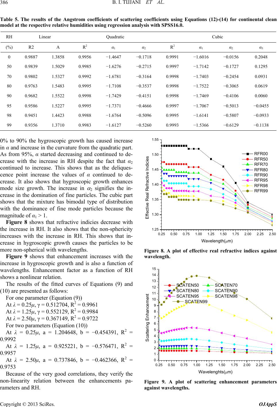

B. I. TIJJANI ET AL. 386
Table 5. The results of the Angstrom coefficients of scattering coefficients using Equations (12)-(14) for continental clean
model at the respective relative humidities using regression analysis with SPSS16.0.
RH Linear Quadratic Cubic
(%) R2 Α R
2 α1 α2 R 2 α1 α2 α3
0 0.9887 1.3858 0.9956 −1.4647 −0.1718 0.9991 −1.6016 −0.0156 0.2048
50 0.9839 1.5029 0.9985 −1.6276 −0.2715 0.9997 −1.7142 −0.1727 0.1295
70 0.9802 1.5327 0.9992 −1.6781 −0.3164 0.9998 −1.7403 −0.2454 0.0931
80 0.9763 1.5483 0.9995 −1.7108 −0.3537 0.9998 −1.7522 −0.3065 0.0619
90 0.9682 1.5522 0.9998 −1.7429 −0.4151 0.9998 −1.7469 −0.4106 0.0060
95 0.9586 1.5227 0.9995 −1.7371 −0.4666 0.9997 −1.7067 −0.5013 −0.0455
98 0.9451 1.4423 0.9988 −1.6764 −0.5096 0.9995 −1.6141 −0.5807 −0.0933
99 0.9356 1.3710 0.9983 −1.6127 −0.5260 0.9993 −1.5366 −0.6129 −0.1138
0% to 90% the hygroscopic growth has caused increase
in α and increase in the curvature from the quadratic part.
As from 95%, α started decreasing and continued to de-
crease with the increase in RH despite the fact that α2
continued to increase. This shows that as the deliques-
cence point increase the values of α continued to de-
crease. It also shows that hygroscopic growth enhances
mode size growth. The increase in 
2 signifies the in-
crease in the domination of fine particles. The cubic part
shows that the mixture has bimodal type of distribution
with the dominance of fine mode particles because the
magnitude of α1 > 1.
0.25 0.50 0.75 1.00 1.25 1.50 1.75 2.00 2.25 2.50
1.25
1.30
1.35
1.40
1.45
1.50
1.55
Effective Real Refractive Indicies
Wavelength(  m)
RFR00
RFR50
RFR70
RFR80
RFR90
RFR95
RFR98
RFR99
Figure 8 shows that refractive indicies decrease with
the increase in RH. It also shows that the non-sphericity
increases with the increase in RH. This shows that in-
crease in hygroscopic growth causes the particles to be
more non-spherical with wavelengths. Figure 8. A plot of effective real refractive indices against
wavelength. Figure 9 shows that enhancement increases with the
increase in hygroscopic growth and is also a function of
wavelengths. Enhancement factor as a function of RH
shows a nonlinear relation.
0.25 0.50 0.75 1.00 1.25 1.50 1.75 2.00 2.25 2.50
0
1
2
3
4
5
6
7
8
9
10
11
12
13
14
15
Scattering Enhancement
Wavelenghts(  m)
SCATEN50 SCATEN70
SCATEN80 SCATEN90
SCATEN95 SCATEN98
SCATEN99
The results of the fitted curves of Equations (9) and
(10) are presented as follows:
For one parameter (Equation (9))
At λ = 0.25μ, γ = 0.512704, R2 = 0.9961
At λ = 1.25μ, γ = 0.552129, R2 = 0.9984
At λ = 2.50μ, γ = 0.367149, R2 = 0.9722
For two parameters (Equation (10))
At λ = 0.25μ, a = 1.204648, b = −0.454391, R2 =
0.9992
At λ = 1.25μ, a = 0.925221, b = −0.576471, R2 =
0.9957
At λ = 2.50μ, a = 0.737846, b = −0.462366, R2 =
0.9753
Because of the very good correlations, they verify the
non-linearity relation between the enhancements pa-
rameters and RH. Figure 9. A plot of scattering enhancement parameters
against wavelengths.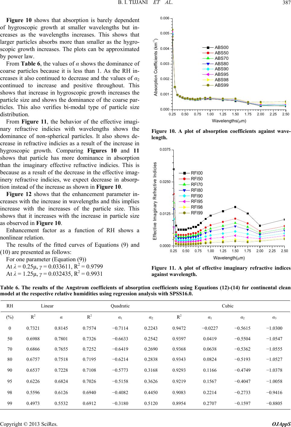

B. I. TIJJANI ET AL. 387
Figure 10 shows that absorption is barely dependent
of hygroscopic growth at smaller wavelengths but in-
creases as the wavelengths increases. This shows that
larger particles absorbs more than smaller as the hygro-
scopic growth increases. The plots can be approximated
by power law.
From Table 6, the values of α shows the dominance of
coarse particles because it is less than 1. As the RH in-
creases it also continued to decrease and the values of α2
continued to increase and positive throughout. This
shows that increase in hygroscopic growth increases the
particle size and shows the dominance of the coarse par-
ticles. This also verifies bi-modal type of particle size
distribution.
From Figure 11, the behavior of the effective imagi-
nary refractive indicies with wavelengths shows the
dominance of non-spherical particles. It also shows de-
crease in refractive indicies as a result of the increase in
hygroscopic growth. Comparing Figures 10 and 11
shows that particle has more dominance in absorption
than the imaginary effective refractive indicies. This is
because as a result of the decrease in the effective imag-
inery refractive indicies, we expect decrease in absorp-
tion instead of the increase as shown in Figure 10.
Figure 12 shows that the enhancement parameter in-
creases with the increase in wavelengths and this implies
increase with the increases of the particle size. This
shows that it increases with the increase in particle size
as observed in Figure 10.
Enhancement factor as a function of RH shows a
nonlinear relation.
The results of the fitted curves of Equations (9) and
(10) are presented as follows:
For one parameter (Equation (9))
At λ = 0.25μ, γ = 0.033611, R2 = 0.9799
At λ = 1.25μ, γ = 0.032435, R2 = 0.9931
0.25 0.50 0.75 1.00 1.25 1.50 1.75 2.00 2.25 2.50
0.000
0.001
0.002
0.003
0.004
0.005
0.006
Absorption Coefficients (km
-1
)
Wavelengths(  m)
ABS00
ABS50
ABS70
ABS80
ABS90
ABS95
ABS98
ABS99
Figure 10. A plot of absorption coefficients against wave-
length.
0.25 0.50 0.75 1.00 1.25 1.50 1.75 2.00 2.25 2.50
0.0000
0.0125
0.0250
0.0375
E ffe ct iv e Imag in a ry R e fra c tiv e Ind ic ie s
Wavelength(  m)
RFI00
RFI50
RFI70
RFI80
RFI90
RFI95
RFI98
RFI99
Figure 11. A plot of effective imaginary refractive indices
against wavelength.
Table 6. The results of the Angstrom coefficients of absorption coefficients using Equations (12)-(14) for continental clean
model at the respective relative humidities using regression analysis with SPSS16.0.
RH Linear Quadratic Cubic
(%) R2 α R2 α1 α2 R
2 α1 α2 α3
0 0.7321 0.8145 0.7574 −0.7114 0.2243 0.9472 −0.0227 −0.5615 −1.0300
50 0.6988 0.7801 0.7326 −0.6633 0.2542 0.9397 0.0419 −0.5504 −1.0547
70 0.6866 0.7655 0.7252 −0.6419 0.2690 0.9368 0.0638 −0.5362 −1.0555
80 0.6757 0.7518 0.7195 −0.6214 0.2838 0.9343 0.0824 −0.5193 −1.0527
90 0.6537 0.7228 0.7108 −0.5773 0.3168 0.9293 0.1166 −0.4749 −1.0378
95 0.6226 0.6824 0.7026 −0.5158 0.3626 0.9219 0.1567 −0.4047 −1.0058
98 0.5596 0.6126 0.6940 −0.4082 0.4450 0.9083 0.2214 −0.2733 −0.9416
99 0.4973 0.5532 0.6912 −0.3180 0.5120 0.8954 0.2707 −0.1597 −0.8805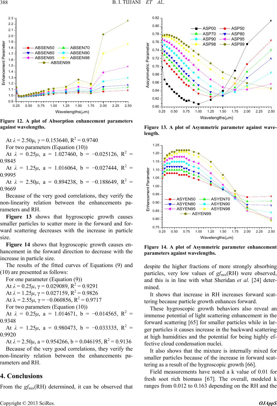

B. I. TIJJANI ET AL. 388
0.25 0.50 0.75 1.00 1.25 1.50 1.75 2.00 2.25 2.50
0.9
1.0
1.1
1.2
1.3
1.4
1.5
1.6
1.7
1.8
1.9
2.0
2.1
2.2
2.3
Enhancement Parameter
Wavelengths(  m)
ABSEN50 ABSEN70
ABSEN80 ABSEN90
ABSEN95 ABSEN98
ABSEN99
Figure 12. A plot of Absorption enhancement parameters
against wavelengths.
At λ = 2.50μ, γ = 0.153640, R2 = 0.9740
For two parameters (Equation (10))
At λ = 0.25μ, a = 1.027460, b = −0.025126, R2 =
0.9845
At λ = 1.25μ, a = 1.016064, b = −0.027444, R2 =
0.9995
At λ = 2.50μ, a = 0.894238, b = −0.188649, R2 =
0.9669
Because of the very good correlations, they verify the
non-linearity relation between the enhancements pa-
rameters and RH.
Figure 13 shows that hygroscopic growth causes
smaller particles to scatter more in the forward and for-
ward scattering decreases with the increase in particle
size.
Figure 14 shows that hygroscopic growth causes en-
hancement in the forward direction to decrease with the
increase in particle size.
The results of the fitted curves of Equations (9) and
(10) are presented as follows:
For one parameter (Equation (9))
At λ = 0.25μ, γ = 0.029089, R2 = 0.9291
At λ = 1.25μ, γ = 0.027159, R2 = 0.9826
At λ = 2.55μ, γ = −0.060856, R2 = 0.9717
For two parameters (Equation (10))
At λ = 0.25μ, a = 1.014671, b = −0.014565, R2 =
0.9348
At λ = 1.25μ, a = 0.980473, b = −0.033335, R2 =
0.9920
At λ = 2.50μ, a = 0.954266, b = 0.046195, R2 = 0.9136
Because of the very good correlations, they verify the
non-linearity relation between the enhancements pa-
rameters and RH.
4. Conclusions
From the gfmix(RH) determined, it can be observed that
0.25 0.50 0.751.001.251.501.75 2.00 2.25 2.50
0.60
0.62
0.64
0.66
0.68
0.70
0.72
0.74
0.76
0.78
0.80
0.82
Assymmetric Parameter
Wavelengths(  m)
ASP00 ASP50
ASP70 ASP80
ASP90 ASP95
ASP98 ASP99
Figure 13. A plot of Asymmetric parameter against wave-
length.
0.25 0.500.75 1.001.25 1.501.75 2.002.25 2.50
0.75
0.80
0.85
0.90
0.95
1.00
1.05
1.10
1.15
1.20
1.25
Enhancement Parameter
Wavelengths(m)
ASYEN50 ASYEN70
ASYEN80 ASYEN90
ASYEN95 ASYEN98
ASYEN99
Figure 14. A plot of Asymmetric parameter enhancement
parameters against wavelengths.
despite the higher fractions of more strongly absorbing
particles, very low values of gfmix(RH) were observed,
and this is in line with what Sheridan et al. [24] deter-
mined.
It shows that increase in RH increases forward scat-
tering because particle growth enhances forward.
These hygroscopic growth behaviors also reveal an
immense potential of light scattering enhancement in the
forward scattering [65] for smaller particles while in lar-
ger particles it causes increase in the backward scattering
at high humidities and the potential for being highly ef-
fective cloud condensation nuclei.
It also shows that the mixture is internally mixed for
smaller particles because of the increase in forward scat-
tering as a result of the hygroscopic growth [66].
Field measurements have noted a k value of 0.01 for
fresh soot rich biomass [67]. The overall, modeled k
ranges from 0.012 to 0.163 depending on the RH and the

B. I. TIJJANI ET AL. 389
type of the mixing ratio used.
Finally, it can be observed that the absorption and
scattering coefficients together with their enhancement
parameters have exponential dependence with RH.
The modeling shows that hygroscopic growth at higher
relative humidity increases the effective radii, scattering
coefficients, scattering enhancement parameters, absorp-
tion coeffeicnts, absorption enhancement parameters, but
decreases effective real refractive indices, effective
imaginary refractive indices. However, the asymmetric
and enhancement asymmetric parameters increase with
the increase in RH but decreases with the increase in
wavelength.
Jeong et al. [10] demonstrated an exponential de-
pendence of the aerosol optical thickness on relative hu-
midity.
Finally, the data fit our models very well and can be
used to extrapolate the hygroscopic growth at any RH
and enhancement parameters at any RH and wavelengths.
The importance of determining gfmix(RH) as a function of
RH and volume fractions, mass fractions and number
fractions, and enhancement parameters as a function of
RH and wavelengths can be potentially important be-
cause it can be used for efficiently representing aero-
sols-water interactions in global models.
REFERENCES
[1] D. A. Randall, R. A. Wood, S. Bony, R. Colman, T. Fi-
chefet, J. Fyfe, V. Kattsov, A. Pitman, J. Shukla, J. Srini-
vasan, R. J. Stouf-fer, A. Sumi and K. E. Taylor, “Con-
tribution of Working Group I to the Fourth Assessment
Report of the Intergovernmental Panel on Climate
Change—Climate Models and their Evaluation,” Cam-
bridge University Press, Cambridge, New York, 2007, pp.
589-662.
[2] D. S. Covert, R. J. Charlson and N. C. Ahlquist, “A Study
of the Relationship of Chemical Composition and Hu-
midity to Light Scattering by Aerosols,” Journal of Ap-
plied Meteorology, Vol. 11, No. 6, 1972, pp. 968-976.
http://dx.doi.org/10.1175/1520-0450(1972)011<0968:AS
OTRO>2.0.CO;2
[3] L. McInnes, M. Bergin, J. Ogren and S. Schwartz, “Ap-
portionment of Light Scattering and Hygroscopic Growth
to Aerosol Composition,” Geophysical Research Letters,
Vol. 25, No. 4, 1998, pp. 513-516.
http://dx.doi.org/10.1029/98GL00127
[4] R. A. Kotchenruther, P. V. Hobbs and D. A. Hegg, “Hu-
midification Factors for Atmospheric Aerosols off the
Mid-Atlantic Coast of the United States,” Journal of
Geophysical Research, Vol. 104, No. D2, 1999, pp. 2239-
2251. http://dx.doi.org/10.1029/98JD01751
[5] W. C. Malm, D. E. Day, S. M. Kreidenweis, J. L. Collett
and T. Lee, “Humidity-Dependent Optical Properties of
Fine Particles during the Big Bend Regional Aerosol and
Visibility Observational Study,” Journal of Geophysical
Research, Vol. 108, No. D9, 2003, p. 4279.
http://dx.doi.org/10.1029/2002JD002998
[6] I. N. Tang, “Chemical and Size Effects of Hygroscopic
Aerosols on Light Scattering Coefficient,” Journal of
Geophysical Research, Vol. 101, No. D14, 1996, pp.
19245-19250. http://dx.doi.org/10.1029/96JD03003
[7] E. Swietlicki, J. Zhou, O. H. Berg, B. G. Martinsson, G.
Frank, S.-I. Cederfelt, U. Dusek, A. Berner, W. Birmilli,
A. Wiedensohler, B. Yuskiewicz and K. N. Bower, “A
Closure Study of Sub-Micrometer Aerosol Particle Hy-
groscopic Behaviour,” Atmospheric Research, Vol. 50 No.
3-4, 1999, pp. 205-240.
http://dx.doi.org/10.1016/S0169-8095(98)00105-7
[8] S. A. Terpugowa, M. V. Panchenko, V. S. Kozlov, V. V.
Polkin and E. P. Yausheva, “The Study of the Growth
Factor of the Aerosol Scattering Coefficient in the Near-
Ground Layer of the Atmosphere in West Siberia,” Euro-
pean Aerosol Conference, Budapest, 2004
[9] J. Kuśmierczyk-Michulec, “Angstrom Coefficient as an
Indicator of the Atmospheric Aerosol Type for a Well-
Mixed Atmospheric Boundary Layer: Part 1: Modelde-
velopment,” Oceanologia, Vol. 51 No. 1, 2009, pp. 5-38.
http://dx.doi.org/10.5697/oc.51-1.005
[10] M. J Jeong, Z. Li, E. Andrews and S. C. Tsay, “Effect of
Aerosol Humidification on the Column Aerosol Optical
Thickness over the Atmospheric Radiation Measurement
Southern Great Plains Site,” Journal of Geophysical Re-
search, Vol. 112, No. D10, 2007, p. 202.
http://dx.doi.org/10.1029/2006JD007176
[11] A. S. Rapti, “Spectral Optical Atmospheric Thickness
Dependence on the Specific Humidity in the Presence of
Continental and Marine Air Masses,” Atmospheric Re-
search, Vol. 78, No. 1-2, 2005, pp. 13-32.
http://dx.doi.org/10.1016/j.atmosres.2005.02.004
[12] Y. Miyazaki, Y. Kondo, N. Takegawa, Y. Komazaki, M.
Fukuda, K. Kawamura, M. Mochida, K. Okuzawa and R.
J. Weber, “Time-Resolved Measurements of Water-Solu-
ble Organic Carbon in Tokyo,” Journal of Geophysical
Research, Vol. 111, No. D23, 2006, p. 206.
http://dx.doi.org/10.1029/2006JD007125
[13] A. P. Sullivan, R. E. Peltier, C. A. Brock, J. A. de Gouw,
J. S. Holloway, C. Warneke, A. G. Wollny and R. J. We-
ber, “Airborne Measurements of Carbonaceous Aerosol
Soluble in Water over Northeastern United States:
Method Development and an Investigation into Wa-
ter-Soluble Organic Carbon Sources,” Journal of Geo-
physical Research, Vol. 111, No. D23, 2006, p. S46.
http://dx.doi.org/10.1029/2006JD007072
[14] Y. Kondo, Y. Miyazaki, N. Takegawa, T. Miyakawa, R. J.
Weber, J. L. Jimenez, Q. Zhang and D. R. Worsnop,
“Oxygenated and Water-Soluble Organic Aerosols in
Tokyo,” Journal of Geophysical Research, Vol. 122, No.
D01, 2007, p. 203.
http://dx.doi.org/10.1029/2006JD007056
[15] R. J. Weber, A. P. Sullivan, R. E. Peltier, A. Russell, B.
Yan, M. Zheng, J. de Gouw, C. Warneke, C. Brock, J. S.
Holloway, E. L. Atlas and E. Edgerton, “A Study of Sec-
ondary Organic Aerosol Formation in the Anthropogenic
Influenced Southeastern United States,” Journal of Geo-
physical Research, Vol. 112, No. D13, 2007, p. 302.

B. I. TIJJANI ET AL. 390
http://dx.doi.org/10.1029/2007JD008408
[16] B. Ervens and R. Volkamer, “Glyoxal Processing by
Aerosol Multiphase Chemistry: Towards a Kinetic Mod-
eling Framework of Secondary Organic Aerosol Forma-
tion in Aqueous Particles,” Atmospheric Chemistry and
Physics, Vol. 10, 2010, pp. 8219-8244.
http://dx.doi.org/10.5194/acp-10-8219-2010
[17] A. Sorooshian, S. M. Murphy, S. Hersey, R. Bahreini, H.
Jonsson, R. C. Flagan and J. H. Seinfeld, “Constraining
the Contribution of Organic Acids and AMS m/z44 to the
Organic Aerosol Budget: On the Importance of Meteor-
ology, Aerosol Hygroscopicity and Region,” Geophysical
Research Letters, Vol. 37, No. 21, 2010.
http://dx.doi.org/10.1029/2010GL044951
[18] H. Timonen, M. Aurela, S. Carbone, K. Saarnio, S.
Saarikoski, T. Makela, M. Kulmala, V. M. Kerminen, D.
R. Worsnop and R. Hillamo, “High Time-Resolution
Chemical Characterization of the Water-Soluble Fraction
of Ambient Aerosols with PILS-TOC-IC and AMS,” At-
mospheric Measurement Techniques, Vol. 3, 2010, pp.
1063-1074. http://dx.doi.org/10.5194/amt-3-1063-2010
[19] K. S. Docherty, E. A. Stone, I. M. Ulbrich, P. F. DeCarlo,
D. C. Snyder, J. J. Schauer, R. E. Peltier, R. J. Weber, S.
M. Murphy, J. H. Seinfeld, D. J. Eatough, B. D. Grover
and J. L. Jimenez, “Apportionment of Primary and Sec-
ondary Organic Aerosols in Southern California during
the 2005 Study of Organic Aerosols in Riverside
(SOAR),” Environmental Science & Technology, Vol. 42,
No. 20, 2008, pp. 7655-7662.
[20] P. McMurry and M. Stolzenburg, “On the Sensitivity of
Particle Size to Relative Humidity for Los Angeles Aero-
sols,” Atmospheric Environment, Vol. 23, No. 2, 1989, pp.
497-507.
http://dx.doi.org/10.1016/0004-6981(89)90593-3
[21] D. Cocker, N. Whitlock, R. Flagan and J. H. Seinfeld,
“Hygroscopic Properties of Pasadena, California Aero-
sol,” Aerosol Science and Technology, Vol. 35, No. 2,
2001, pp. 637-647.
http://dx.doi.org/10.1080/02786820120653
[22] E. Swietlicki, et al., “Hygroscopic Properties of Submi-
crometer Atmospheric Aerosol Particles Measured with H
TDMA Instruments in Various Environments—A Re-
view,” Tellus B, Vol. 60, No. 3, 2008, pp. 432-469.
http://dx.doi.org/10.3402/tellusb.v60i3.16936
[23] H. Kohler, “The Nucleus and Growth of Hygroscopic
Droplets,” Transactions of the Faraday Society, Vol. 32,
1936, pp. 1152-1161.
http://dx.doi.org/10.1039/tf9363201152
[24] P. J. Sheridan, D. J. Delene and J. A. Ogren, “Four Years
of Continuous Surface Aerosol Measurements from the
Department of Energy’s Atmospheric Radiation Meas-
urement Program Southern Great Plains Cloud and Ra-
diation Testbedsite,” Journal of Geophysical Research,
Vol. 106, No. 20, 2001, pp. 735-747.
http://dx.doi.org/10.1029/2001JD000785
[25] M. Hess, P. Koepke and I. Schult, “Optical Properties of
Aerosols and Clouds: The Software Package OPAC,”
Bulletin of the American Meteorological Society, Vol. 79,
No. 5, 1998, pp. 831-844.
[26] C. A. Randles, L. M. Russell and V. Ramaswamy, “Hy-
groscopic and Optical Properties of Organic Sea Salt
Aerosol and Consequences for Climate Forcing,” Geo-
physical Research Letters, Vol. 31, No. 16, 2004, Article
ID: L16108. http://dx.doi.org/10.1029/2004GL020628
[27] P. F. Liu, C. S. Zhao, T. Gobel, E. Hallbauer, A. Nowak,
L. Ran, W. Y. Xu, Z. Z. Deng, N. Ma, K. Mildenberger, S.
Henning, F. Stratmann and A. Wiedensohler, “Hygro-
scopic Proper Ties of Aerosol Particles at High Relative
Humidity and Their Diurnal Variations in the North
China Plain,” Atmospheric Chemistry and Physics, Vol.
11, 2011, pp. 2991-3040.
http://dx.doi.org/10.5194/acpd-11-2991-2011
[28] G. Buzorius, A. Zelenyuk, F. Brechtel and D. Imre, “Si-
multaneous Determination of Individual Ambient Particle
Size, Hygroscopicity and Composition,” Geophysical Re-
search Letters, Vol. 29, 1974, 2002.
http://dx.doi.org/10.1029/2001GL014221
[29] S. Sjogren, M. Gysel, E. Weingartner, U. Baltensperger,
M. J. Cubison, H. Coe, A. A. Zardini, C. Marcolli, U. K.
Krieger and T. Peter, “Hygroscopic Growth and Water
Uptake Kinetics of Two-Phase Aerosol Particles Consist-
ing of Ammonium Sulfate, Adipic and Humic Acid Mix-
tures,” Journal of Aerosol Science, Vol. 38, No. 2, 2007,
157-171. http://dx.doi.org/10.1016/j.jaerosci.2006.11.005
[30] R. H. Stokes and R. A. Robinson, “Interactions in Aque-
ous Nonelec-trolyte Solutions. I. Solute-Solvent Equilib-
ria,” The Journal of Physical Chemistry, Vol. 70, No. 7,
1966, pp. 2126-2130.
http://dx.doi.org/10.1021/j100879a010
[31] N. K. Meyer, J. Duplissy, M. Gysel, A. Metzger, J. Dom-
men, E. Weingartner, M. R. Alfarra, A. S. H. Prevot, C.
Fletcher, N. Good, G. McFiggans, A. M. Jonsson, M.
Hallquist, U. Baltensperger and Z. D. Ristovski, “Analy-
sis of the Hy-groscopic and Volatile Properties of Am-
monium Sulphate Seeded and Unseeded SOA Particles,”
Atmospheric Chemistry and Physics, Vol. 9, 2009, pp.
721-732. http://dx.doi.org/10.5194/acp-9-721-2009
[32] M. Stock, Y. F. Cheng, W. Birmili, A. Massling, B. Weh-
ner, T. Muller, S. Leinert, N. Kalivitis, N. Mihalopoulos
and A. Wiedensohler, “Hygroscopic Properties of At-
mospheric Aerosol Particles over the Eastern Mediterra-
nean: Implications for Regional Direct Radiative Forcing
under Clean and Polluted Conditions,” Atmospheric
Chemistry and Physics, Vol. 11, 2011, pp. 4251-4271.
www.atmos-chem-phys.net/11/4251/2011/
http://dx.doi.org/10.5194/acp-11-4251-2011
[33] J. Duplissy, P. F. DeCarlo, J. Dommen, M. R. Alfarra, A.
Metzger, I. Barmpadimos, A. S. H. Prevot, E. Weingart-
ner, T. Tritscher, M. Gysel, A. C. Aiken, J. L. Jimenez, M.
R. Canagaratna, D. R. Worsnop, D. R. Collins, J. Tom-
linson and U. Baltensperger, “Relating Hygroscopicity
and Composition of Organic Aerosol Particulate Matter,”
Atmospheric Chemistry and Physics, Vol. 11, 2011, pp.
1155-1165.
www.atmos-chem-phys.net/11/1155/2011/
http://dx.doi.org/10.5194/acp-11-1155-2011
[34] J. Meier, B. Wehner, A. Massling, W. Birmili, A. Nowak,
T. Gnauk, E. Bruggemann, H. Herrmann, H. Min and A.
Wiedensohler, “Hygroscopic Growth of Urban Aerosol

B. I. TIJJANI ET AL. 391
Particles in Beijing (China) during Wintertime: A Com-
parison of Three Experimental Methods,” Atmospheric
Chemistry and Physics, Vol. 9, 2009, pp. 6865-6880.
www.atmos-chem-phys.net/9/6865/2009/
http://dx.doi.org/10.5194/acp-9-6865-2009
[35] M. D. Petters and S. M. Kreidenweis, “A Single Parame-
ter Representation of Hygroscopic Growth and Cloud
Condensation Nucleus Activity,” Atmospheric Chemistry
and Physics, Vol. 7, No. 8, 2007, pp. 1961-1971.
http://dx.doi.org/10.5194/acp-7-1961-2007
[36] J. H. Seinfeld and S. N. Pandis, “Atmospheric Chemistry
and Physics,” Wiley-Interscience Publication, Hoboken,
1998.
[37] J. Seinfeld and S. Pandis, “Atmospheric Chemistry and
Physics,” 2nd Edition, Wiley-Interscience, New York,
2006.
[38] E. Swietlicki, J. Zhou, D. S. Covert, K. Hameri, B. Busch,
M. Vakeva, U. Dusek, O. H. Berg, A. Wiedensohler, P.
Aalto, J. Makela, B. G. Martinsson, G. Papaspiropoulos,
B. Mentes, G. Frank and F. Stratmann, “Hygroscopic Pro-
perties of Aerosol Particles in the Northeastern Atlantic
during ACE-2,” Tellus, Vol. 52, No. 2, 2000, pp. 201-
227.
[39] W. Birmili, A. Nowak, K. Schwirn, K. Lehmann, et al.,
“A New Method to Accurately Relate Dry and Humidi-
fied Number Size Distributions of Atmospheric Aero-
sols,” Journal of Aerosol Science, Vol. 1, No. 1, 2004, pp.
15-16.
[40] F. Kasten, “Visibility Forecast in the Phase of Pre-Con-
densation,” Tellus, Vol. 21, No. 5, 1969, pp. 631-635.
[41] M. Gysel, G. B. McFiggans and H. Coe, “Inversion of
Tandem Differential Mobility Analyser (TDMA) Meas-
urements,” Journal of Aerosol Science, Vol. 40, No. 2,
2009, pp. 134-151.
http://dx.doi.org/10.1016/j.jaerosci.2008.07.013
[42] J.-P. Putaud, “Interactive Comment on ‘Aerosol Hygro-
scopicity at Ispra EMEP-GAW Station’ by M. Adam et
al.,” Atmospheric Chemistry and Physics Discussions,
Vol. 12, No. 1, 2012, pp. C200-C202.
[43] S. I. Christensen and M. D. Petters, “The Role of Tem-
perature in Cloud Droplet Activation,” The Journal of
Physical Chemistry A, Vol. 116, No. 39, 2012, pp. 9706-
9717. http://dx.doi.org/10.1021/jp3064454
[44] S. J. Doherty, et al., “A Comparison and Summary of Ae-
rosol Optical Properties as Observed in Situ from Air-
craft, Ship, and Land during ACE-Asia,” Journal of Geo-
physical Research: Atmospheres, Vol. 110, No. D4, 2005,
Article ID: D04201.
http://dx.doi.org/10.1029/2004JD004964
[45] P. K. Quinn, et al., “Impact of Particulate Organic Matter
on the Relative Humidity Dependence of Light Scattering:
A Simplified Parameterization,” Geophysical Research
Letters, Vol. 32, No. 22, 2005, Article ID: L22809.
http://dx.doi.org/10.1029/2005GL024322
[46] S. Gasso, et al., “Influence of Humidity on the Aerosol
Scattering Coefficient and Its Effect on the Upwelling Ra-
diance during ACE-2,” Tellus B, Vol. 52, No. 2, 2000, pp.
546-567.
[47] A. Clarke, et al., “Biomass Burning and Pollution Aero-
sol over North America: Organic Components and Their
Influence on Spectral Optical Properties and Humidifica-
tion Response,” Journal of Geophysical Research: At-
mospheres, Vol. 112, No. D12, 2007, Article ID: D12S18.
http://dx.doi.org/10.1029/2006JD007777
[48] G. Hanel, “The Properties of Atmospheric Aerosol Parti-
cles as Functions of Relative Humidity at Thermody-
namic Equilibrium with Surrounding Moist Air,” In: H. E.
Landsberg and J. Van Mieghem, Eds., Advances in Geo-
physics, Academic Press, New York, 1976, pp. 73-188.
[49] M. K. Latha and K. V. S. Badarinath, “Factors Influen-
cing Aerosol Characteristics over Urban Environment,”
Environmental Monitoring and Assessment, Vol. 104, No.
1-3, 2005, pp. 269-280.
http://dx.doi.org/10.1007/s10661-005-1615-7
[50] A. Angstrom, “Techniques of Determining the Turbidity
of the Atmosphere,” Tellus, Vol. 13, No. 2, 1961, pp. 214-
223.
http://dx.doi.org/10.1111/j.2153-3490.1961.tb00078.x
[51] M. D. King and D. M. Byrne, “A Method for Inferring
Total Ozone Content from Spectral Variation of Total
Optical Depth Obtained with a Solar Radiometer,” Jour-
nal of the Atmospheric Sciences, Vol. 33, No. 11, 1976,
pp. 2242-2251.
http://dx.doi.org/10.1175/1520-0469(1976)033<2242:AM
FITO>2.0.CO;2
[52] T. F. Eck, B. N. Holben, J. S. Reid, O. Dubovic, A.
Smirnov, N. T. O’Neil, I. Slutsker and S. Kinne, “Wave-
length Dependence of the Optical Depth of Biomass Bur-
ning, Urban, and Desert Dust Aerosols,” Journal of Geo-
physical Research: Atmospheres, Vol. 104, No. D24,
1999, pp. 31333-31349.
[53] T. F. Eck, B. N. Holben, O. Dubovic, A. I. Smirnov, J.
Slutsker, M. Lobert and V. Ramanathan, “Column-Inte-
grated Aerosol Optical Properties over the Maldives dur-
ing the Northeast Mon-Soon for 1998-2000,” Journal of
Geophysical Research: Atmospheres, Vol. 106, 2001, pp.
28555-28566.
[54] T. F. Eck, B. N. Holben, D. E. Ward, O. Dubovic, J. S.
Reid, A. Smirnov, M. M. Mukelabai, N. C. Hsu, N. T. O’
Neil and I. Slutsker, “Characterization of the Optical Pro-
perties of Biomass Burning Aerosols in Zambia during
the 1997 ZIBBEE Field Campaign,” Journal of Geophy-
sical Research: Atmospheres, Vol. 106, No. D4, 2001, pp.
3425-3448. http://dx.doi.org/10.1029/2000JD900555
[55] Y. J. Kaufman, “Aerosol Optical Thickness and Atmos-
pheric Path Radiance,” Journal of Geophysical Research:
Atmospheres, Vol. 98, No. D2, 1993, pp. 2677-2992.
http://dx.doi.org/10.1029/92JD02427
[56] N. T. O’Neill, O. Dubovic and T. F. Eck, “Modified Ån-
gström Exponent for the Characterization of Submicro-
meter Aerosols,” Applied Optics, Vol. 40, No. 15, 2001,
pp. 2368-2375.
http://dx.doi.org/10.1364/AO.40.002368
[57] N. T. O’Neill, T. F. Eck, A. Smirnov, B. N. Holben and S.
Thulasiraman, “Spectral Discrimination of Coarse and Fine
Mode Optical Depth,” Journal of Geophysical Research:
Atmospheres, Vol. 108, No. D17, 2003.

B. I. TIJJANI ET AL. 392
[58] R. Pedros, J. A. Martinez-Lozano, M. P. Utrillas, J. L.
Gomez-Amo and F. Tena, “Column-Integrated Aerosol,
Optical Properties from Ground-Based Spectroradiometer
Measurements at Barrax (Spain) during the Digital Air-
borne Imaging Spectrometer Experiment (DAISEX) Cam-
paigns,” Journal of Geophysical Research: Atmospheres,
Vol. 108, No. D18, 2003, pp. 1-12.
http://dx.doi.org/10.1029/2002JD003331
[59] D. G. Kaskaoutis and H. D. Kambezidis, “Investigation
on the Wavelength Dependence of the Aerosol Optical
Depth in the Athens Area,” Quarterly Journal of the
Royal Meteorological Society, Vol. 132, No. 620, 2006,
pp. 2217-2234. http://dx.doi.org/10.1256/qj.05.183
[60] B. Schmid, D. A. Hegg, J. Wang, D. Bates, J. Redemann,
P. B. Russell, J. M. Livingston, H. H. Jonsson, E. J. Wel-
ton, J. H. Seinfeld, R. C. Flagan, D. S. Covert, O. Dubo-
vik and A. Jefferson, “Column Closure Studies of Lower
Tropospheric Aerosol and Water Vapor during ACE-Asia
Using Airborne Sun Photometer and Airborne in Situ and
Ship-Based Lidar Measurements,” Journal of Geophysi-
cal Research: Atmospheres, Vol. 108, No. D23, 2003, pp.
1-19. http://dx.doi.org/10.1029/2002JD003361
[61] J. A. Martinez-Lozano, M. P. Utrillas, F. Tena, R. Pedros,
J. Canada, J. V. Bosca and J. Lorente, “Aerosol Optical
Characteristics from Summer Campaign in an Urban Coas-
tal Mediterranean Area,” IEEE Transactions on Geosci-
ence and Remote Sensing, Vol. 39, No. 7, 2001, pp. 1573-
1585. http://dx.doi.org/10.1109/36.934089
[62] D. E. Aspens, “Local-Field Effect and Effective Medium
Theory: A Microscopic Perspective,” American Journal
of Physics, Vol. 50, No. 8, 1982, pp. 704-709.
http://dx.doi.org/10.1119/1.12734
[63] H. A. Lorentz, “Ueber Die Beziehungzwischen der Fortp-
flanzungsgeschwindigkeit des Lichtes und der Körperdi-
chte,” Annalen der Physik, Vol. 245, No. 4, 1880, pp.
641-665. http://dx.doi.org/10.1002/andp.18802450406
[64] L. Lorenz, “Ueber Die Refractionconstante,” Annalen der
Physik, Vol. 11, No. 1, 1880, pp. 70-103.
[65] K. N. Liou, “An Introduction to Atmospheric Radiation,”
Elsevier, New York, 2002.
[66] J. Wang and S. T. Martin, “Satellite Characterization of
Urban Aerosols: Importance of Including Hygroscopicity
and Mixing State in the Retrieval Algorithms,” Journal of
Geophysical Research: Atmospheres, Vol. 112, No.
D17203, 2007, pp. 1-18.
http://dx.doi.org/10.1029/2006JD008078
[67] M. O. Andreae and D. Rosenfeld, “Aerosol-Cloud-Pre-
cipitation Interactions. Part 1. The Nature and Sources of
Cloud-Active Aerosols,” Earth-Science Reviews, Vol. 89,
No. 1-2, 2008, pp. 13-41.
http://dx.doi.org/10.1016/j.earscirev.2008.03.001
[68] T. F. Eck, B. N. Holben, D. E. Ward, M. M. Mukelabai,
O. Dubovik, A. Smirnov, J. S. Schafer, N. C. Hsu, S. J.
Piketh, A. Queface, J. Le Roux, R. J. Swap and I. Slutsker,
“Variability of Biomass Burning Aerosol Optical Char-
acteristics in Southern Africa during the SAFARI 2000
Dry Season Campaign and a Comparison of Single Scat-
tering Albedo Estimates from Radiometric Measure-
ments,” Journal of Geophysical Research: Atmosphere,
Vol. 108, No. D13, 2003, pp.
[69] G. L. Schuster, O. Dubovik and B. N. Holben, “Angstrom
Exponent and Bimodal Aerosol Size Distributions,”
Journal of Geophysical Research: Atmosphere, Vol. 111,
No. D17, 2006, Article ID: D07207.
http://dx.doi.org/10.1029/2005JD006328
[70] D. G. Kaskaoutis, H. D. Kambezidis, N. Hatzianastassiou,
P. G. Kosmopoulos and K. V. S. Badarinath, “Aerosol
Climatology: Dependence of the Angstrom Exponent on
Wavelength over Four AERONET Sites,” Atmospheric
Chemistry and Physical Discussion, Vol. 7, No. 3, 2007,
pp. 7347-7397.
http://dx.doi.org/10.5194/acpd-7-7347-2007
[71] D. G. Kaskaoutis, H. D. Kambezidis, N. Hatzianastassiou,
P. G. Kosmopoulos and K. V. S. Badarinath, “Aerosol
Climatology: On the Discrimination of Aerosol Types
over four AERONET Sites,” Atmospheric Chemistry and
Physical Discussion, Vol. 7, No. 3, 2007, pp. 6357-6411.
http://dx.doi.org/10.5194/acpd-7-6357-2007
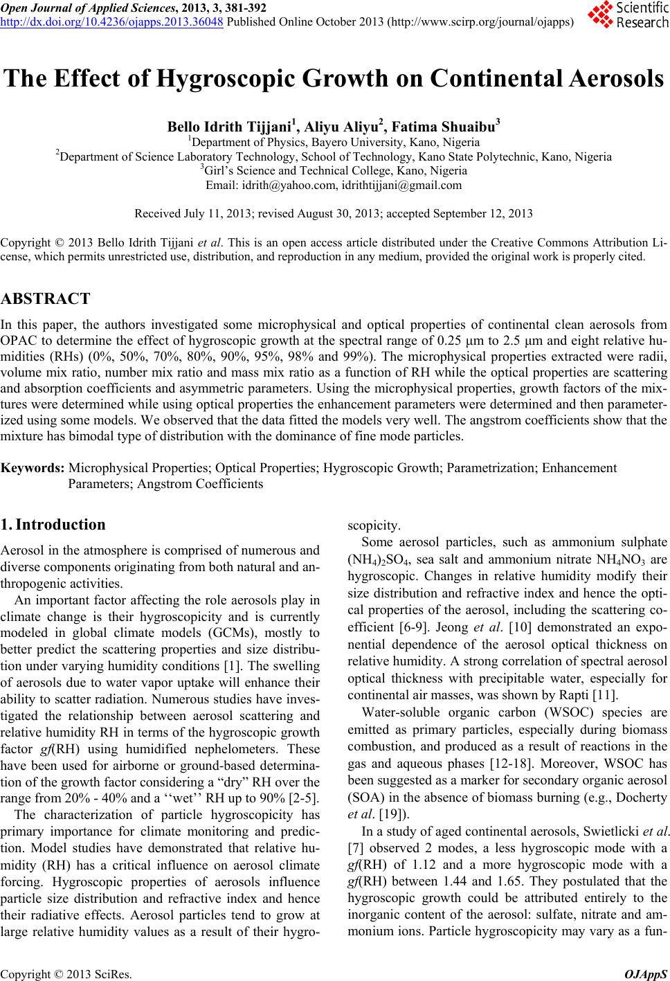