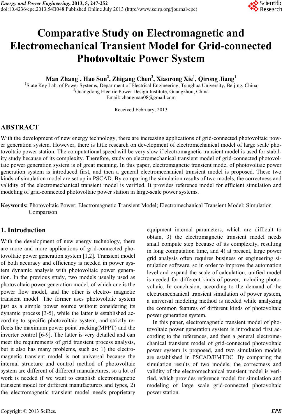Energy and Power E ngineering, 2013, 5, 247-252
doi:10.4236/epe.2013.54B048 Published Online July 2013 (http://www.scirp .o rg/journal/epe)
Comparative Study on Electromagnetic and
Electr omechanical Transient Model for Grid-connected
Photovoltaic Pow er System
Man Zhang1, Hao Sun2, Zhigang Chen2, Xiaorong Xie1, Qirong Jiang1
1State Key Lab. of Po wer Systems, Dep ar tment of Electri cal Engin eer ing, Tsinghua University, Beijing, China
2Guangdong Electric Power Design Institute, Guangzhou, China
Received February, 2013
ABSTRACT
With t he de vel op ment o f ne w ene rg y tech nolo gy, the re a re increasing applicatio ns of grid-connected photovoltaic pow-
er generation system. However, there is little research on development of electromechanical model of large scale pho-
tovoltaic power station. The computatio nal sp eed will be ve ry slo w if electr o magnetic tra nsient model is u sed for stabil-
it y st ud y becau se of its complexity. Therefore, study on electromecha nical transient model of grid-connected photovol-
taic power generation system is of great meaning. In this paper, electromagnetic transient model of photovoltaic power
generation system is introduced first, and then a general electromechanical transient model is proposed. These two
kinds of simulation model are set up in PSCAD. By comparing the simulation results of two models, the correctness and
validity of the electromechanical transient model is verified. It provides reference model for efficient simulation and
modeling of grid-connected photovoltaic power station in large-scale power systems.
Keywords: Photovoltaic Power; Electromag netic Transient Model; Electromechanical Transient Model; Simulation
Comparison
1. Introduction
With the development of new energy technology, there
are more and more applications of grid-connected pho-
tovoltaic po wer generatio n syste m [1,2]. Transient model
of both accuracy and efficiency is needed in power sys-
tem dynamic analysis with photovoltaic power genera-
tion. In the previous study, two models usually used as
photovoltaic power generation model, of which one is the
power flow model, and the other is electro- magnetic
transient model. The former uses photovoltaic system
just as a simple power source without considering its
dynamic process [3-5], while the latter is established ac-
cording to specific photovoltaic system, and strictly re-
flects the maximum power point tracking(MPPT ) and the
inverter control [6-9]. The latter is very detailed and can
meet the requirements of grid transient process analysis,
but it also has many problems, such as: 1) the electro-
magnetic transient model is not universal because the
internal structure and control method of photovoltaic
syst em are diffe rent of di ffere nt manufactures, so a lot of
work is needed if we want to establish electromagnetic
transient model for different manufacturers and types, 2)
the electromagnetic transient model needs proprietary
equipment internal parameters, which are difficult to
obtain, 3) the electromagnetic transient model needs
small compute step because of its complexity, resulting
in long computation time, and 4) at present, large power
grid analysis often requires business or engineering si-
mulation software, so in order to improve the automation
level and expand the scale of calculation, unified model
is needed for different kinds of power, including photo-
voltaic. In conclusion, according to the demand of the
electromechanical transient simulation of power system,
a universal modeling method is needed while analyzing
the common features of different kinds of photovoltaic
power generation system.
In this paper, electromagnetic transient model of pho-
tovoltaic power generation system is introduced first ac-
cording to the references, and then a general electrome-
chanical transient model of grid-connected photovoltaic
power system is proposed, and two simulation models
are established in PSCAD/EMTDC. By comparing the
simulation results of two models, the correctness and
validity of the electromechanical transient model is veri-
fied, which provides reference model for simulation and
modeling of large scale grid-connected photovoltaic
po wer station.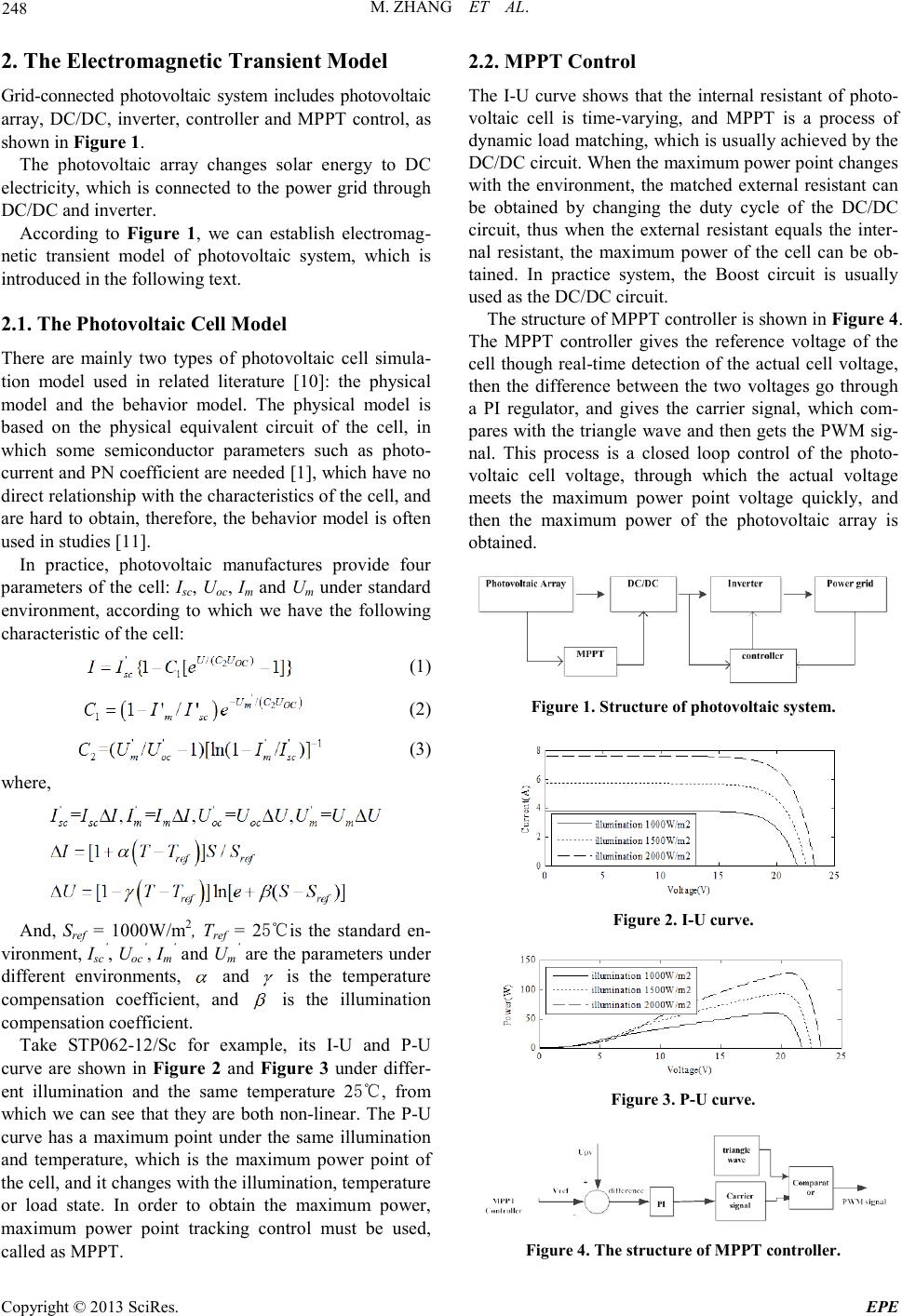

M. ZH AN G ET AL.
248
2. The Electromagnetic Transient Model
Grid-connected photovoltaic system includes photovol taic
array, DC/DC, inverter, controller and MPPT control, as
sho wn in Figure 1.
The photovoltaic array changes solar energy to DC
electricity, which is connected to the power grid through
DC/DC and inverter.
According to Figure 1, we can establish electromag-
netic transient model of photovoltaic system, which is
introduced in the following text.
2.1. The Photovoltaic Cell Model
There are mainly two types of photovoltaic cell simula-
tion model used in related literature [10]: the physical
model and the behavior model. The physical model is
based on the physical equivalent circuit of the cell, in
which some semiconductor parameters such as photo-
current and PN coefficient are needed [1] , which have no
direct re lationship with the characteristics of the cell, and
are hard to obtain, therefore, the behavior model is often
used in studies [11].
In practice, photovoltaic manufactures provide four
parameters of the cell: Isc, Uoc, Im and Um under standard
environment, according to which we have the following
characteristic of the cell:
(1)
(2)
(3)
where,
And, Sref = 1000W/m2, Tref = 25℃is the standard en-
vironment, Isc’, Uoc’, Im’ and Um’ are the parameters under
different environments, and is the temperature
compensation coefficient, and is the illumination
compensatio n co e fficient.
Take STP062-12/Sc for example, its I-U and P-U
curve are shown in Figure 2 and Figure 3 under differ-
ent illumination and the same temperature 25℃, from
which we can see that they are both non-linear. The P-U
curve has a maximum point under the same illumination
and temperature, which is the maximum power point of
the cell, and it changes with th e illumination, temperature
or load state. In order to obtain the maximum power,
maximum power point tracking control must be used,
called as MPPT.
2.2. MPPT Control
The I-U curve shows that the internal resistant of photo-
voltaic cell is time-varying, and MPPT is a process of
dynamic load matching, whic h is us uall y achi eve d by the
DC/DC circuit. When the max i mu m power po i nt cha n ge s
with the environment, the matched external resistant can
be obtained by changing the duty cycle of the DC/DC
circuit, thus when the external resistant equals the inter-
nal resistant, the maximum power of the cell can be ob-
tained. In practice system, the Boost circuit is usually
used as the DC/DC circuit.
The structure of MPPT co nt rol ler is sho wn i n Figure 4.
The MPPT controller gives the reference voltage of the
cell though real-time detection of the actual cell voltage,
then the difference between the two voltages go through
a PI regulator, and gives the carrier signal, which com-
pares with the triangl e wave and then gets the PWM sig-
nal. This process is a closed loop control of the photo-
voltaic cell voltage, through which the actual voltage
meets the maximum power point voltage quickly, and
then the maximum power of the photovoltaic array is
obtained.
Figure 1 . Structure of photovoltaic syst em.
Figure 2. I-U curve.
Figure 3. P-U curve.
Figure 4. T he structure of MPPT controller.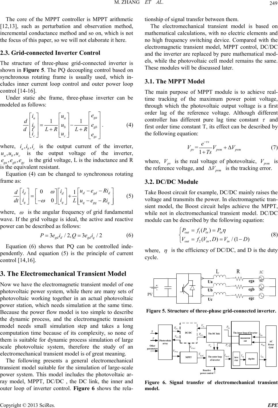

M. ZH AN G ET AL.
249
The core of the MPPT controller is MPPT arithmetic
[12,13], such as perturbation and observation method,
incremental conductance method and so on, which is not
the focus of this paper, so we will not elaborate it here.
2.3. Grid-connected Inverter Control
The structure of three-phase grid-connected inverter is
sho wn i n Figure 5. The PQ decoupling control based on
synchronous rotating frame is usually used, which in-
cludes inner current loop control and outer power loop
control [14-16].
Under static abc frame, three-phase inverter can be
modeled as follows:
11
ga
aa
bb gb
cc
gc
e
iu
diue
dt LRLR
iue

 
 
=− 
 
++

 
 
. (4)
where,
,,
abc
i ii
is the output current of the inverter,
,,
abc
u uu
is the output voltage of the inverter,
,,
ga gb gc
eee
is the gr id vo lta ge, L is the ind ucta nce a nd R
is the equivale nt re sistant.
Equation (4) can be changed to synchronous rotating
frame as:
01
0
d gdd
dd
qq
q gqq
u eRi
ii
d
ii
u eRi dt L
ω
ω
−−

 

=+ 
 

− −−
 
 
(5)
where,
ω
is the angular frequency of grid fundamental
wave. If the grid voltage is ideal, the active and reactive
power can be described as follows:
3/2, 3/2
gd dgd q
P eiQei= =
(6)
Equation (6) shows that PQ can be controlled inde-
pendently. And equation (5) is the principle of current
control [14,16].
3. The Electromechanical Transient Model
Now we have the electromagnetic transient model of one
photovoltaic power system, while there are many sets of
photovoltaic working together in an actual photovoltaic
power station, which needs simulation at the same time.
Because the power flow model is too simple to describe
the dynamic process, and the electromagnetic transient
model needs small simulation step and takes a long
computation time because of its complexity, so none of
them is suitable for dynamic process simulation of large
scale photovoltaic system, therefore the study of an
electromechanical transient model is of great meaning.
The following presents a general electromechanical
transient model suitable for the simulation of large-scale
power system. This model includes the photovoltaic ar-
ray model, MPPT, DC/DC , the DC link, the inner and
outer loop of inverter control. Figure 6 shows the rela-
tionship of signal transfer between them.
The electromechanical transient model is based on
mathematical calculations, with no electric elements and
no high frequency switching device. Compared with the
electromagnetic transient model, MPPT control, DC/DC
and the inverter are replaced by pure mathematical mod-
els, while the photovoltaic cell model remains the same.
These modules will b e discussed la te r.
3.1. The MPPT Model
The main purpose of MPPT module is to achieve real-
time tracking of the maximum power point voltage,
through which the photovoltaic output voltage is a first
order lag of the reference voltage. Although different
controller has different pure lag time constant
τ
and
first order ti me constant T, its e ffect can be described b y
the followin g eq uation:
=1
s
pvpvm pvm
e
V VV
Ts
τ −
+∆
+
(7)
where,
pv
V
is the real voltage of photovoltaic,
pvm
V
is
the reference voltage, and
pvm
V∆
is the tracking error.
3.2. DC/DC Module
Take Boo st circuit for exa mple, DC/DC main ly raise s the
voltage and transmits the power. In electromagnetic tran-
sient model, the Boost circuit helps achieve the MPPT,
while not in electromechanical transient model. DC/DC
module can be described by the follo wing equation:
1
2
()
(,)/ (1)
outin in
out inin
PfP P
VfV DVD
η = =

== −

(8)
where,
η
is the efficiency of DC/D C, and D is the duty
cycle.
AC
AC
AC
LR
Ua
Ub
Uc
ega
egb
egc
PV
Figure 5. Structure of three-phase grid-connected invert er.
The inner loop of inverter
The outer loop
of inverter
MPPT
Photovoltaic
array
S
T
Other
parameters
PV1
P
PV1
V
PVm
V
DC/DC
D,ref
V
The DC link
PV2
P
D
V
dq,ref
I
D
V
PVm1
V
Reactive
power control
De
P
abc
i
abc
u
inve
rter
dq
I
dq/abc
measurem
ent
,
ee
PQ
abc
i
AC
Power
Grid
Figure 6. Signal transfer of electromechanical transient
mode l .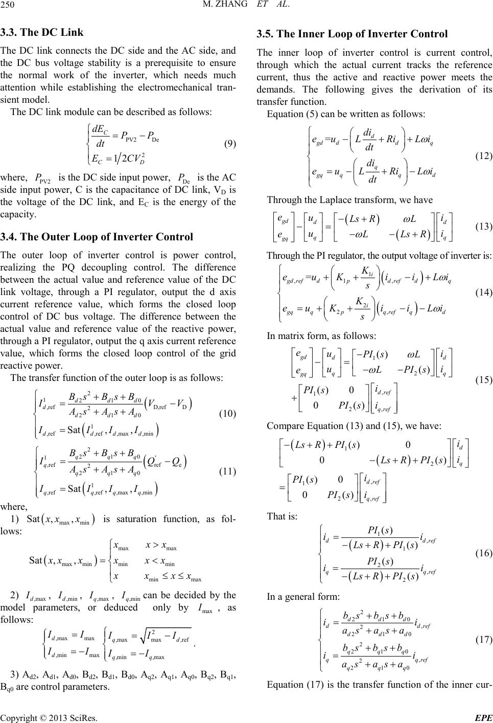

M. ZH AN G ET AL.
250
3.3. The DC Link
The DC link connects the DC side and the AC side, and
the DC bus voltage stability is a prerequisite to ensure
the normal work of the inverter, which needs much
attention while establishing the electromechanical tran-
sient model.
The DC link module can be described as follows:
PV2 De
2
12
C
CD
dE PP
dt
E CV
= −


=

(9)
where,
PV2
P
is the DC side inp ut po wer,
De
P
is the AC
side input power, C is the capacitance of DC link, VD is
the voltage of the DC link, and EC is the energy of the
capacity.
3.4. The Outer Loop of Inverter Control
The outer loop of inverter control is power control,
realizing the PQ decoupling control. The difference
between the actual value and reference value of the DC
link voltage, through a PI regulator, output the d axis
current reference value, which forms the closed loop
control of DC bus voltage. The difference between the
actual value and reference value of the reactive power,
thro ugh a P I re gula to r , o utp ut t he q axi s c ur r ent r e fer e nc e
value, which forms the closed loop control of the grid
reactive power.
The transfer fu nction of the outer loop is as follows:
( )
( )
2
12 10
,refD,ref D
2
2 10
1
,ref,ref,max,min
Sat, ,
d dd
d
d dd
ddd d
BsBs B
I VV
AsAs A
III I
++
= −

++

=


(10)
( )
( )
2
2 10
1'
,refref e
2
2 10
1
,ref,ref,max ,min
Sat,,
q qq
q
q qq
qqq q
BsBs B
I QQ
AsAs A
III I
++
= −

++

=


(11)
where,
1)
( )
max min
Sat ,,xx x
is saturation function, as fol-
lows:
( )
max max
max minminmin
min max
Sat,,
x xx
xxxxx x
xx xx
>


= <

≤≤

2)
,maxd
I
,
,mind
I
,
,maxq
I
,
,minq
I
can be decided by the
model parameters, or deduced only by
max
I
, as
follows:
2
,max max,maxmax ,ref
,minmax ,min ,max
dqd
dqq
II
I II
II
II

=
= −


= −= −


.
3) Ad2, Ad1, Ad0, Bd2, Bd1, Bd0, Aq2, Aq1, Aq0, Bq2, Bq1,
Bq0 are control parameters.
3.5. The Inner Loop of Inverter Control
The inner loop of inverter control is current control,
through which the actual current tracks the reference
current, thus the active and reactive power meets the
demands. The following gives the derivation of its
transfer function.
Equation (5) c a n b e written as follows:
=
d
gd ddq
q
gq qqd
di
euLRiL i
dt
di
euLRiL i
dt
ω
ω

− ++




=− +−



(12)
Through t he Laplace transform, we ha ve
( )
( )
gd
dd
qq
gq
e
ui
Ls RL
ui
LLs R e
ω
ω
  
− +
−=
  

− −+


   (13)
Through the PI regulator, the output voltage of inverter is:
( )
( )
1
, 1,
2
2,
=
i
gd refdpd refdq
i
gqqpqrefqd
K
euKiiLi
s
K
e uKii Li
s
ω
ω

+ +−+

 

=++−−



(14)
In matrix form, as follows:
1
2
,
1
2,
()
()
() 0
0 ()
gd
dd
qq
gq
d ref
q ref
e
ui
PI sL
ui
LPI s e
i
PI s
PI si
ω
ω

  −

−=
  

−−


 



+




(15)
Compare Equation (13) and (15), we have:
( )
( )
1
2
,
1
2,
() 0
0 ()
() 0
0 ()
d
q
d ref
q ref
i
LsRPI s
i
LsRPI s
i
PI s
PI si

−+ +

− ++
 


=




That is:
( )
( )
1,
1
2,
2
()
()
()
()
dd ref
qq ref
PI s
ii
LsRPI s
PI s
ii
LsRPI s
=
− ++


=
− ++

(16)
In a general form:
2
2 10
,
2
2 10
2
2 10
,
2
2 10
d dd
dd ref
d dd
q qq
qq ref
q qq
bsbs b
ii
asas a
bsbs b
ii
asasa
++
=
++

++
=
++

(17)
Equation (17) is the transfer funct ion of the inner cur-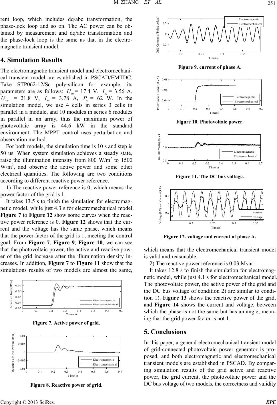

M. ZH AN G ET AL.
251
rent loop, which includes dq/abc transformation, the
phase-lock loop and so on. The AC power can be ob-
tained by measurement and dq/abc transformation and
the phase-lock loop is the same as that in the electro-
magnetic transient model.
4. Simulation Results
The electromagnetic transient model a nd electromechani-
cal transient model are established in PSCAD/EMT DC.
Take STP062-12/Sc poly-silicon for example, its
parameters are as follows: m
U= 17.4 V,
m
I
= 3.56 A,
oc
U
= 21.8 V,
sc
I
= 3.78 A,
m
P
= 62 W. In the
simulation model, we use 4 cells in series 3 cells in
parallel in a module, and 10 modules in series 6 modules
in parallel in an array, thus the maximum power of
photovoltaic array is 44.6 kW in the standard
environment. The MPPT control uses perturbation and
observation method.
For both models, the simulation time is 10 s and step is
50 us. When system simulation achieves a steady state,
raise the illumination intensity from 800 W/m2 to 1500
W/m2, and observe the active p ower and some other
electrical quantities. The following are two conditions
according to different reactive power reference.
1) The reactive power reference is 0, which means the
power factor of the grid is 1.
It takes 13.5 s to finish the simulation for electromag-
netic model, while just 4.3 s fo r electromechanical model.
Figure 7 to Figure 12 sho w some curves when the reac-
tive power reference is 0. Figure 12 shows that the cur-
rent and the voltage has the same phase, which means
that the power factor of the grid is 1, meeting the control
goal. From Figure 7, Figure 9, Figure 10, we can see
that the photovoltaic p ower, t he active and reactive pow-
er of the grid increase after the illumination density in-
creases. In addition, Figure 7 to Figure 11 sho w that the
simulations results of two models are almost the same,
00.1 0.2 0.3 0.4 0.5 0.6 0.7
0.03
0.04
0.05
0.06
0.07
Time(s)
Active Gr id Po we r ( M VA)
Elect r o m agnetic
Elect r o m echanical
Figure 7. Active power of grid.
00.1 0.2 0.30.4 0.5 0.60.7
-0.01
-0.005
0
0.005
0.01
Time ( s)
Reactive o f Gr id Po wer( M v ar )
Electro magnet ic
Electro mechanical
Figure 8. Reactive power of grid.
0.2 0.25 0.3 0.35
-0.2
0
0.2
Time ( s)
Grid Current of Pahse A(kA)
Electro m agnetic
Electro m echan ical
Figure 9. current of phase A.
00.1 0.2 0.3 0.4 0.5 0.6 0.7
0.04
0.06
0.08
Time ( s)
Photov olta ic Powe r (MV A)
Electro m agnetic
Electro m echan ical
Figure 1 0. Photovoltaic power.
00.1 0.2 0.30.4 0.50.6 0.7
0.8
0.9
1
Time ( s)
DC Bus Vo ltag e( kV)
Electro m agnetic
Electro m echan ical
Figure 11. The DC bus voltage.
0.2 0.25 0.3 0 .35
-0.2
0
0.2
Time ( s)
Voltage(kV) and Current(kA)
curr en t
voltage
Figure 1 2. voltage and current of phase A .
which means that the electromechanical transient model
is valid and reasonable.
2) The reactive power reference is 0.03 Mvar.
It takes 12.8 s to finish the simulation for electromag-
netic model, while just 4.1 s fo r electromechanical model.
The photovoltaic power, the active power of the grid and
the DC bus voltage of condition 2) are similar to condi-
tion 1). Figure 13 shows the reactive power of the grid,
and Figure 14 shows the current and voltage, between
which the phase is not the same but has an angle, mea n-
ing that the grid power factor is not 1.
5. Conclusions
In this paper, a general electro mechanical tra nsient model
of grid-connected photovoltaic power generator is pro-
posed, and both electromagnetic and electromechanical
transient models are established in PSCAD. By co mpar-
ing simulation results of the grid active and reactive
power, the grid current, the photovoltaic power and the
DC bus volt age of two model s , the correctne s s and validit y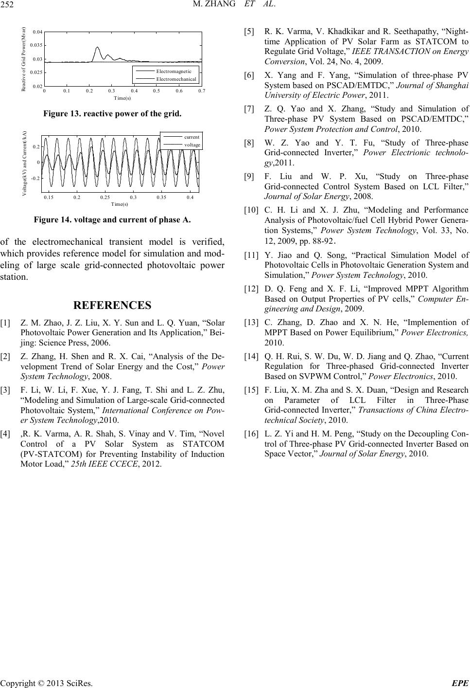

M. ZH AN G ET AL.
252
00.1 0.2 0.30.4 0.50.6 0.7
0.02
0.025
0.03
0.035
0.04
Time ( s)
Reactive o f Gr id Po wer( M v ar )
Electro m agnetic
Electro m echan ical
Figure 1 3. reactive power of the grid.
0.15 0.2 0.250.3 0.35 0.4
-0.2
0
0.2
Time ( s)
Voltage(kV) and Current(/kA)
curr en t
volt age
Figure 1 4. voltage and current of phase A .
of the electromechanical transient model is verified,
which provides reference model for simulation and mod-
eling of large scale grid-connected photovoltaic power
station.
REFERENCES
[1] Z. M. Zhao, J. Z. Liu, X. Y. Sun and L. Q. Yuan, “Solar
Photovoltaic Power Generation and Its Application,” Bei-
jing: Science Pres s , 2006.
[2] Z. Zhang, H. Shen and R. X. Cai, “Analysis of the De-
velopment Trend of Solar Energy and the Cost,” Power
System Technology, 2008.
[3] F. Li, W. Li, F. Xue, Y. J. Fang, T. Shi and L. Z. Zhu,
“Modeling and Simulation of Large-scale Grid-connected
Photovoltaic S yste m,” International Conference on Pow-
er System Technology,2010.
[4] ,R. K. Varma, A. R. Shah, S. Vinay and V. Tim, “Novel
Control of a PV Solar System as STATCOM
(PV-STATCOM) for Preventing Instability of Induction
Motor Load,” 25th IEEE CCECE, 2012.
[5] R. K. Varma, V. Khadkikar and R. Seethapathy, “Night-
time Application of PV Solar Farm as STATCOM to
Regulate Grid Voltage,” IEEE TRANSACTION on Energy
Conversion , Vol. 24, No. 4, 2009.
[6] X. Yang and F. Yang, “Simulation of three-phase PV
System based on PSCAD/EMTDC,” Journal of Shanghai
Universi ty of Electric Power, 2011.
[7] Z. Q. Yao and X. Zhang, “Study and Simulation of
Three-phase PV System Based on PSCAD/EMTDC,”
Power System Protec t ion and Control, 2010.
[8] W. Z. Yao and Y. T. Fu, “Study of Three-phase
Grid-connected Inverter,” Power Electrionic technolo-
gy,2011.
[9] F. Liu and W. P. Xu, “Study on Three-phase
Grid-connected Control System Based on LCL Filter,”
Journal of Solar Energy, 2008.
[10] C. H. Li and X. J. Zhu, “Modeling and Performance
Analysis of Photovoltaic/fuel Cell Hybrid Power Genera-
tion Sys t e m s ,” Power System Technology, Vol. 33, No.
12, 2009, pp. 88-92．
[11] Y. Jiao and Q. Song, “Practical Simulation Model of
Photovoltaic Cells in Photovoltaic Generation System and
Simulation,” Power System Technology, 20 10 .
[12] D. Q. Feng and X. F. Li, “Improved MPPT Algorithm
Based on Output Properties of PV cells,” Computer En-
gineering and Design, 2009 .
[13] C. Zhang, D. Zhao and X. N. He, “I mp l e me ntion of
MPPT Based on Power Equilibrium,” Power Electro nics,
2010.
[14] Q. H. Rui, S. W. Du, W. D. Jiang and Q. Zhao, “Current
Regulation for Three-phased Grid-connected Inverter
Based on SVPWM Control,” Power Electronics, 2010.
[15] F. Liu, X. M . Zha an d S. X. Du an , “Design and Research
on Parameter of LCL Filter in Three-Phase
Gri d-co nnected In verter,” Transactions of China Electro-
technical Society, 2010.
[16] L. Z. Yi and H. M. Peng, “Study on the Decoupling Con-
trol of Three-phase P V Grid-conn ected Inverter Based on
Space Vector,” Journ al of Solar Ener gy, 2010.