W. H. WANG ET AL.
Copyright © 2013 SciRes. OJCE
00.5 11.5 22.5 3
0
0.5
1
1.5
2
x/H
Cs
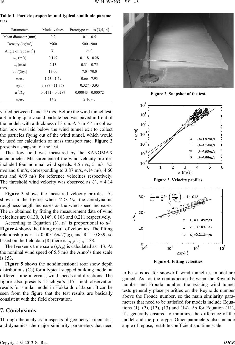
Tsuchiya-1
Tsuchiya-2
Tsuchiya-3
t
= 300s,
U
= 4.60m/s,
β
= 0
o
t
= 300s,
U
= 4.99m/s,
β
= 0
o
t
= 300s,
U
= 5.36m/s,
β
= 0
o
t
= 300s,
U
= 4.99m/s,
β
= 15
o
t
= 900s,
U
= 4.99m/s,
β
= 15
o
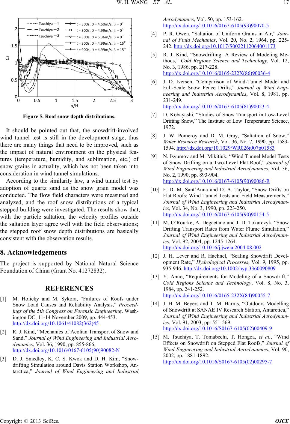
Figure 5. Roof snow depth distr i but ions.
It should be pointed out that, the snowdrift-involved
wind tunnel test is still in the development stage, thus
there are many things that need to be improved, such as
the impact of natural environment on the physical fea-
tures (temperature, humidity, and sublimation, etc.) of
snow grains in actuality, which has not been taken into
consideration in wind tunnel simulations.
According to the similarity law, a wind tunnel test by
adoption of quartz sand as the snow grain model was
conducted. The flow field characters were measured and
analyzed, and the roof snow distributions of a typical
stepped building were investigated. The results show that,
with the particle saltation, the velocity profiles outside
the saltation layer agree well with the field observations;
the stepped roof snow depth distributions are basically
consistent with the observation results.
8. Acknowledgements
The project is supported by National Natural Science
Foundation of Chi na ( G rant No. 41 272832) .
REFERENCES
[1] M. Holicky and M. Sykora, “Failures of Roofs under
Snow Load Causes and Reliability Analysis,” Proceed-
ings of the 5th Congress on Forensic Engineering, Wash-
ington DC, 11-14 November 2009, pp. 444-453.
http://dx.doi.org/10.1061/41082(362)45
[2] R. J. Kind, “Mechanics of Aeolian Transport of Snow and
Sand,” Journal of Wind Engineering and Industrial Aero-
dynamics, Vol. 36, 1990, pp. 855-866.
http://dx.doi.org/10.1016/0167-6105(90)90082-N
[3] D. J. Smedley, K. C. S. Kwok and D. H. Kim, “Snow-
drifting Simulation around Davis Station Workshop, An-
tarctica,” Journal of Wind Engineering and Industrial
Aerodynamics, Vol. 50, pp. 153-162.
http://dx.doi.org/10.1016/0167-6105(93)90070-5
[4] P. R. Owen, “Saltation of Uniform Grains in Air,” Jour-
nal of Fluid Mechanics, Vol. 20, No. 2, 1964, pp. 225-
242. http://dx.doi.org/10.1017/S0022112064001173
[5] R. J. Kind, “Snowdrifting: A Review of Modeling Me-
thods,” Cold Regions Science and Technology, Vol. 12,
No. 3, 1986, pp. 217-228.
http://dx.doi.org/10.1016/0165-232X(86)90036-4
[6] J. D. Iversen, “Comparison of Wind-Tunnel Model and
Full-Scale Snow Fence Drifts,” Journal of Wind Engi-
neering and Industrial Aerodynamics, Vol. 8, 1981, pp.
231-249.
http://dx.doi.org/10.1016/0167-6105(81)90023-4
[7] D. Kobayashi, “Studies of Snow Transport in Low-Level
Drifting Snow,” The Institute of Low Temperature Science,
1972.
[8] J. W. Pomeroy and D. M. Gray, “Saltation of Snow,”
Water Resource Research, Vol. 36, No. 7, 19 90, pp. 1583-
1594. http://dx.doi.org/10.1029/WR026i007p01583
[9] N. Isyumov and M. Mikitiuk, “Wind Tunnel Model Tests
of Snow Drifting on a Two-Level Flat Roof,” Journal of
Wind Engineering and Industrial Aerodynamics, Vol. 36,
No. 2, 1990, pp. 893-904.
http://dx.doi.org/10.1016/0167-6105(90)90086-R
[10] F. D. M. Sant’Anna and D. A. Taylor, “Snow Drifts on
Flat Roofs: Wind Tunnel Tests and Field Measurements,”
Journal of Wind Engineering and Industrial Aerodynam-
ics, Vol. 34, No. 3, 1990, pp. 223-250.
http://dx.doi.org/10.1016/0167-6105(90)90154-5
[11] M. O’Rourke, A. Degaetano and J. D. Tokarczyk, “Snow
Drifting Transport Rates from Water Flume Simulation,”
Journal of Wind Engineering and Industrial Aerodynam-
ics, Vol. 92, 2004, pp. 1245-1264.
http://dx.doi.org/10.1016/j.jweia.2004.08.002
[12] J. H. Lever and R. Haehnel, “Scaling Snowdrift Devel-
opment Rate,” Hydrological Processes, Vol. 9, 1995, pp.
935-946. http://dx.doi.org/10.1002/hyp.3360090809
[13] Y. Anno, “Requirements for Modeling of a Snowdrift,”
Cold Regions Science and Technology, Vol. 8, No. 3,
1984, pp. 241-252.
http://dx.doi.org/10.1016/0165-232X(84)90055-7
[14] J. H. M. Beyers and T. M. Harms, “Outdoors Modelling
of Snowdrift at SANAE IV Research Station, Antarctica,”
Journal of Wind Engineering and Industrial Aerodynam-
ics, Vol. 91, 2003, pp. 551-569.
http://dx.doi.org/10.1016/S0167-6105(02)00409-9
[15] M. Tsuchiya, T. Tomabechi, T. Hongoa, et al., “Wind
Effects on Snowdrift on Stepped Flat Roofs,” Journal of
Wind Engineering and Industrial Aerodynamics, Vol. 90,
2002, pp. 1881-1892.
http://dx.doi.org/10.1016/S0167-6105(02)00295-7