Communications and Network, 2013, 5, 601-605
http://dx.doi.org/10.4236/cn.2013.53B2108 Published Online September 2013 (http://www.scirp.org/journal/cn)
Threshold Selection Study on Fisher Discriminant Analysis
Used in Exon Prediction for Unbalanced Data Sets
Yutao Ma1, Yanbing Fang2, Ping Liu1, Jianfu Teng3
1School of Physics and Electrical Information Engineering, Ningxia University, Yinchuan, China
2School of Mathematics and Computer Science, Ningxia University, Yinchuan, China
3School of Electronic Information Engineering, Tianjin University, Tianjin, China
Received May 2013
ABSTRACT
In gene prediction, the Fisher discriminant analysis (FDA) is used to separate protein coding region (exon) from non-
coding regions (intron). Usually, the positive data set and the negative data set are of the same size if the number of the
data is big enough. But for some situations the data are not sufficient or not equal, the threshold used in FDA may have
important influence on prediction results. This paper presents a study on the selection of the threshold. The eigen value
of each exon/intron sequence is computed using the Z-curve method with 69 variables. The experiments results suggest
that the size and the standard deviation of the data sets and the threshold are the three key elements to be taken into
consideration to improve the prediction results.
Keywords: Fisher Discriminant Analysis; Threshold Selection; Gene Prediction; Z-Curve; Size of Data Set
1. Introduction
Protein coding region and non-coding region of a DNA
sequence are also called exon and intron respectively.
Gene prediction of eukaryotes is still one of the most
important research domains of bioinformatics for the
prediction accuracy is needed to be improved [1]. Fisher
Discriminant analysis/algorithm (FDA) is widely used in
solving binary classification problems like fault classifi-
cation [2], gene expression data classification [3], image
categorization [4], integrating heterogeneous data sets [5]
and DNA sequence classification [6,7], and it has at-
tracted more and more attention. Kernel FDA (KFDA)
may present out performance in both simulation time
consume and classification precision than support vector
machine (S VM) for i t does not need t o solve any quadratic
problem [8,9]. For maximizing the uniformity of class-
pair separabilities and class separability in kernel space
simultaneously, a novel kernel FDA kernel parameters
optimization criterion is presented [10]. A novel dimen-
sionality reduction algorithm based on FDA is proposed
for ranking applications such as visual search re-ranking
[11].
Usually, the size of the training and test data sets are
selected equal and the threshold is determined by making
the false negative rate and the false positive rate equal [6];
but for some real situations, the threshold could not be
obtained by the method because the sizes of the positive
and negative data sets are unbalanced. In the latter situa-
tion, there are five possible thresholds for making the
coding/non-coding decision. Using the exon and intron
data sets downloaded from the website:
http://www.fruitfly.org/seq_tools/datasets/Human/, the FDA
based experiments show that the size and the standard
deviation of the data sets are the two key elements to be
taken into consideration to improve the prediction re-
sults.
2. Data Sets and Methods
2.1. The Data Sets
The Data sets used in this paper were downloaded from
the above net address. The Data were separated into 7
parts in the website, and each part consists of an exon
sub-set and an intron sub-set. There are 301 DNA frag-
ments at least an d 448 at most in each sub-set as detailed
in Table 1.
The difference values between the numbers of exons
and introns in each part are all 66 from the Table 1.
Table 1. The details of each part of the data sets.
Part0 Part1 Part2 Part3 Part4 Part5 Part6
Exon 367 448 447 389 399 402 391
Intron 301 382 381 323 333 336 325
Total 668 830 828 712 732 738 716

Y.-T. MA ET AL.
602
2.2. The Z Curve Methods
The Z curve method is a powerful tool to visualize and
analyze DNA sequences. It is also one of the most widely
used mapping methods which maps a DNA sequence
into three digital sequences. According to [6], the predic-
tion results of the Z curve method with 69 variables are
almost the same with that of 169 variables ones. So, the
Z curve method with 69 variables is applied in this paper.
The 69 variables are composed with 9 Z curve parame-
ters for frequencies of phase-specific mononucleotides,
12 Z curve parameters for frequencies of phase indepen-
dent di-nucleotides and 48 Z curve parameters for fre-
quencies of phase independent tri-nucleotides. These Z
curve parameters are defined below.
Let A, T, C and G represent base adenine, thymine,
cytosine and guanine respectively. The bases A, T, C, G
are occurr ing in a DNA fragment at positions 1, 4, 7, …;
2, 5, 8, …; and 3, 6, 9, …, with frequencies
1
a
,
1
t
,
1
c
,
1
g
;
2
a
,
2
t
,
2
c
,
2
g
;
3
a
,
3
t
,
3
c
,
3
g
respectively.
Then by using the Z-transform defined by Equation (1), a
fragment of DNA sequence is transformed into the 9 Z
curve parameters for frequencies of phase-specific mo-
nonucleotides.
()( )
()( )
( )()
,,[1, 1 ],1,2,3
ii iii
ii iii
iiii i
iii
x agct
y acgt
z atgc
xyz i
= +−+

=+−+

= +− +

∈− =
. (1)
Let
()p XY
be the frequency of the di-nucleotides
XY
(
, CGTXY A=,,,
), the 12 variables for frequen-
cies of phase independent di-nucleotides are given by
[ ()()][ ()()]
[ ()()][ ()()]
[ ()()][ ()()]
,,,
X
X
X
xpXApXGp XCP XT
ypXApXCp XGP XT
zpXAp XTp XGP XC
XACGT
=+−+

=+− +

=+−+

=
. (2)
The last 48 Z curve parameters for frequencies of
phase independent tri-nucleotides can be obtained using
the similar notations by
[ ()()][ ()()]
[ ()()][ ()()]
[ ()()][()()]
,,,, ,,,
XY
XY
XY
xp XYAp XYGp XYCPXYT
yp XYApXYCp XYGP XYT
zp XYAp XYTp XYGP XYC
XACGT YAC GT
=+−+

=+− +

=+−+

= =
. (3)
Next, the 6 9 variabl e s of each exon/intron are
999 12 1212 484848
129 1212 1248
,,,,,,,,, ,,uuuuuuuuu 
. They are
defined by Equations (4) to (8). These
99 9
112233
99 9
4 15263
99 9
7 18293
,,,
,,,
,,
uxuxux
uyuyuy
uzuzuz
= ==
= ==
= ==
. (4)
121212 12
1 234
1212 12 12
5 678
12 12 1212
910 11 12
, , ,,
,,,,
,,,
AC GT
AC GT
ACG T
uxuxuxux
uyuyuyuy
uzuzuzuz
=== =
== = =
= = ==
. (5)
48 4848 48
1234
4848 48 48
5678
48 484848
910 11 12
48 484848
13 141516
,,,,
,, ,,
,,,,
,,,,
AAACAG AT
CACCCG CT
GA GCGG GT
TA TCTGTT
uxuxuxux
uxuxuxux
uxuxuxux
uxuxuxux
= == =
== = =
= ===
= ===
. (6)
48 4848 48
17 1819 20
4848 4848
2122 2324
48 484848
25 262728
48 484848
29 303132
,,,,
,, ,,
,,,,
, ,,,
AAACAG AT
CACC CG CT
GA GC GGGT
TATCTG TT
uyuyuyuy
uyuyuyuy
uyuyuyuy
uyuyuyuy
= ===
= = = =
= ===
= ===
. (7)
48 484848
33 343536
48484848
37383940
48 484848
41 424344
48 484848
45 464748
,,,,
,,,,
,,,,
,,,.
AAACAG AT
CACC CG CT
GA GC GGGT
TATC TG TT
uzuzuzuz
uzuzuzuz
uzuzuzuz
uzuzuzuz
= == =
== ==
= ===
= ===
. (8)
2.3. The Fisher Discriminant Analysis/Algorithm
Let
NM
R
×
∈X
be the data matrix, where N and M are
the number of data/samples and the dimension of each
data respectively. The M is also the number of the best
FDA coefficients, which are
12
,,,
M
uu u
. In this paper
the dimension of the data is 69, that is
69M=
. Each
exon/Intron is described by a point or row vector
x
in a
69-dimensional (69-D) spa c e spanned by
999 121212 484848
129 1212 1248
1 269
(,,,,,,,,, ,, )
(, ,,)
T
T
uuuu uuu uu
xx x
=
=
x 

,
(9)
There are two groups of samples in the training data
set used in FDA. One contains positive samples which
belong to sample space
p w
, and another contains the
negative samples which belong to sample space
n w
. The
positive samples are DNA fragments from real exons and
the negative samples are from the real introns. All the
sequences longer than 2000 bases were cut down to 2000
bases. The numbers of positive and negative samples are
p N
and
n N
respectively, and
pnNNN= +
. The mean
vector of the positive/negative samples in input space is
defined by
n
11
, ,,
MM
pn pn
pn
RR
NN
∈∈
==∈∈
∑∑
p
xw xw
ux uxuu
. (10)
The best FDA coefficients consists a column vector
u
.
Using the divergence matrix W
S, the vector
u
is defined
as the best projecting direc tion (BP D ) a n d i s given by
( )
( )
( )
1
12
,,, ,
TM
pn
MW
uu uR
−
== −∈uSuuu
, (11)
where “T” indicates the transpose of a matrix, and the

Y.-T. MA ET AL.
603
divergence matrix
W
S
is defined as
( )( )
2
,
j
T
W ijij
jpni N= ∈
= −−
∑∑
Sxu xu
. (12)
Once the
u
and the threshold
c
are obtained, the dis-
crimination of exon/intron for each DNA fragment in the
test set is carried out by
00
TT
cc•−> •−<ux ux
.
2.4. The Threshold Selection of FDA
For situations where numbers of positive and negative
samples are not equal, in other words
pn NN≠
, there are
five different thresholds (
1
c
,

,
5
c
) to be selected,
which are represented by Equations (13) to (17).
( )
1
2
Tpn
c+ =uu u
, (13)
( )
2
Tpp nn
NN
cN
+
=uu u
, (14)
( )
3
Tnppn
NN
cN
+
=uu u
, (15)
( )
4
Tpp nn
pn
c
σσ
σσ
+
=+
uuu


, (16)
where
p σ

and
n σ 
are the average variances of the
positive and negative samples respectively.
( )
5
Tnp pn
pn
c
σσ
σσ
+
=+
uu u


. (17 )
For situation where
pn NN=
, the threshold is uniquely
determined by letting the false negative rate (FNR) be
equal to the false positive rate (FPR) [6,7]. The details
will be given in the next section of this paper.
2.5. The Z Curve Mark of th e DNA Sequence
The best projecting direction
u
can be interpreted as the
weight vector corresponds to the 69 Z curve values of
each test sample. The Z curve score (ZCS) of each DNA
sequence is defined as
ZCM = ×ux
, where the “×” is
the multiplication cross symbol, “
u
”and “
x
” are the best
project direction and row vector of a DNA sequence. The
ZCS is too small to be display directly, so a transform
named remainder and multiple (RM) is carried out. The
RM transform is defined as
()(1000, )
()(1000 /)
R ZCSMODZCSM
MZCSfloorZCSM
= ×
= ×
, (18)
where “MOD” and “floor” are two MATLAB function
names. Function “mod(x, y)” returns the modulus of “x”
after it is devided by “y”, and function “floor(x)” rounds
the elements of “x” to the nearest integers. In this work,
the “M” in the RM transform is set to 3. Thus, the ZCS
of a DNA sequence can be displayed in a two dimen-
sional surface with the rounds (
()M ZCS
) and the mod-
ulus (
()R ZCS
) are the two coordinate axis.
3. Results and Discussion
3.1. The Prediction Accuracy Measures
To measure the prediction accuracy, the sensitivity and
the specificity are applied. They are defined by Equations
(19) and (20) respectively.
/ ()100%
n
STP TP FN= +×
(19)
/ ()100%
p
STNTN FP= +×
(20)
where
TPTN
is the number of true exons/introns which
were predicted as exons/introns, and the FP/FN is the
number of true introns/exons which were predicted as
exons/introns [12]. The prediction average accuracy is
defined as
()
np
aSS= +
. The FPR and the FNR are de-
fined by Eq ua tions (20) and (21) respectively.
1/( )
p
FPRSFP TNFP=−=+
(21)
1/( )
n
FNRSFNTP FN=−= +
(22)
Let
FPR FNR=
, we have
()()FP TNFPFNTPFN+= +
.
For the situation
pN
equals to
nN
, the expressions
n NTN FP= +
and
p NTP FN= +
are satisfied. Then we
have
FP FN=
, and the threshold can be expressed as
() ( )
0
/ /2
TT
ppnnp n c NNN=+=+uuuuu u
. (23)
The Statistics of the ZCS of Data Sets.
To clear the relationship between the data sets and the
prediction results, the statistics nature of the 7 data parts
are presented in Tables 2 and 3. These statistics nature
include mean and standard deviation of the Z curve value.
Figure 1 gives the ZCS scatter diagram of the Part0 to
Part6 with the RM transform is applied to the ZCS of
each sequence.
Table 2. The ZCS statistics nature of the exon sequences.
Data sets Part0 Part1 Part2 Part3 Part4 Part5 Part6
mean 0.0053 0.0039 0.0043 0.0035 0.0043 0.0053 0.0043
SDa 0.0053 0.0043 0.0039 0.0043 0.0044 0.0045 0.0041
Table 3. The ZCS statistics nature of the intron sequences.
Data
sets Part0 Part1 Part2 Part3 Part4 Part5 Part6
mean −0.0103 −0.0086 −0.0055 −0.0078 −0.0075 −0.0065 −0.0064
SDa 0.0041 0.0034 0.0028 0.0036 0.0034 0.0033 0.0035

Y.-T. MA ET AL.
604
Figure 1. The ZCS scatter diagram of the data set.
3.2. Test with Different Training/Testing Sets
To study the relationship between size of the training
samples and the prediction results, two experiments wer e
carried out. In the first experiment, let part0 be the train-
ing data set (TRDS) and th e rest 6 parts together (NPart0)
be the test data set (TEDS) at first. Then let part1 be the
training set and the rest 6 parts together (NPart1) be the
test set, and so on. Table 4 gives the prediction results.
Table 5 shows the mean prediction resu lts obtained with
the different training and testing sets (according to Table
4) for the five thresholds. It is clear that the fifth thre-
shold (c5) is the best choice in this experiment situation,
c3 is the next choice except c5, and the c1 is the third
choice.
From the mean prediction accuracies listed in the Ta-
ble 5, the third and the fifth thresholds present a little
better prediction than the three others.
In the second experiment, let the part0 be the training
set (1Parts) at first, and then let the part0 and the part1
(2Parts)be the training set, and so on. In this experiment,
the testing set includes all the seven parts. Table 6 gives
the prediction r esult using the c5 as the threshold. Figure
2 shows the BPD obtained with training sets as men-
tioned like 1Parts, 2Parts, etc. The BPDs changed greatly
as the size of training data set increased, which is con-
firmed by the prediction accuracy listed in Table 6. The
mean and standard deviation of the Z curve value in
Tables 2 and 3 also show the same correlation.
Table 4. Prediction results with different training sets.
Threshold
TRDS Part0 Part1 Part2 Part3 Part4 Part5 Part6
TEDS NPart0 NPart1 NPart2 NPart3 NPart4 NPart5 NPart6
NS 4556 4394 4396 4512 4492 4486 4508
c1
Sn (%) 86.19 85.51 87.90 89.28 88.22 85.70 89.07
Sp (%) 97.89 97.94 97.95 95.93 97.82 97.89 96.51
a (%) 91.99 91.68 92.85 92.38 92.94 91.75 92.61
c2
Sn (%) 83.00 82.38 85.60 87.49 85.88 83.08 86.87
Sp (%) 98.61 98.40 98.61 96.93 98.73 98.69 97.48
a (%) 90.80 90.39 92.08 92.09 92.28 90.88 92.10
c3
Sn (%) 88.65 87.68 89.40 91.2 90.38 87.67 90.62
Sp (%) 96.74 97.13 97.19 94.35 96.89 96.75 95.12
a (%) 92.55 92.29 93.15 92.34 93.46 92.07 92.54
c4
Sn (%) 82.27 81.88 83.01 87.61 84.98 80.58 87.07
Sp (%) 98.69 98.54 98.76 96.76 98.81 99.14 97.44
a (%) 90.49 90.21 90.88 92.06 91.88 89.88 92.17
c5
Sn (%) 89.22 88.68 90.82 91.04 90.96 89.27 90.54
Sp (%) 96.25 96.81 96.33 94.42 96.61 95.61 95.24
a (%) 92.54 92.59 93.33 92.31 93.57 92.19 92.57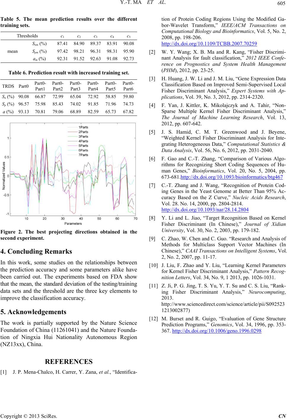

Y.-T. MA ET AL.
605
Table 5. The mean prediction results over the different
training sets.
Thresholds c1 c2 c3 c4 c5
mean
Snm (%) 87.41 84.90 89.37 83.91 90.08
Spm (%) 97.42 98.21 96.31 98.31 95.90
am (%) 92.31 91.52 92.63 91.08 92.73
Table 6. Prediction result with increased training set.
TRDS Part0 Part0-
Part1 Part0- Part2 Part0- Part3 Part0- Part4 Part0- Part5 Part0- Part6
Sn (%) 90.08 66.87 72.99 65.04 72.92 58.85 59.80
Sp (%) 96.57 75.98 85.43 74.02 91.85 71.96 74.73
a (%) 93.13 70.81 79.06 68.89 82.59 65.73 67.82
Figure 2. The best projecting directions obtained in the
second experiment.
4. Concluding Remarks
In this work, some studies on the relationships between
the prediction accuracy and some parameters alike have
been carried out. The experiments based on FDA show
that the mean, the standard deviation of the testing/training
data sets and the threshold are the three key elements to
improve the classification accuracy.
5. Acknowledgements
The work is partially supported by the Nature Science
Foundation of China (11261041) and the Nature Founda-
tion of Ningxia Hui Nationality Autonomous Region
(NZ13xx), China.
REFERENCES
[1] J. P. Mena-Chalco, H. Carrer, Y. Zana, et al., “Identifica-
tion of Protein Coding Regions Using the Modified Ga-
bor-Wavelet Transform,” IEEE/ACM Transactions on
Computational Biology and Bioinformatics, Vol. 5, No. 2,
2008, pp. 198-206.
http://dx.doi.org/10.1109/TCBB.2007.70259
[2] W. Y. Wang; X. B. Ma and R. Kang, “Fisher Discrimi-
nant Analysis for fault classification,” 2012 IEEE Confe-
rence on Prognostics and System Health Management
(PHM), 2012, pp. 23-25.
[3] H. Huang, J. W. Li and J. M. Liu, “Gene Expression Data
Classification Based on Improved Semi-Supervised Local
Fisher Discriminant Analysis,” Expert Systems with Ap-
plications, Vol. 39, No. 3, 2012, pp. 2314-2320.
[4] F. Yan, J. Kittler, K. Mikolajczyk and A. Tahir, “Non-
Sparse Multiple Kernel Fisher Discriminant Analysis,”
The Journal of Machine Learning Research, Vol. 13,
2012, pp. 607-642.
[5] J. S. Hamid, C. M. T. Greenwood and J. Beyene,
“Weighted Kernel Fisher Discriminant Analysis for Inte-
grating Heterogeneous Data,” Computational Statistics &
Data Analysis, Vol. 56, No. 6, 2012, pp. 2031-2040.
[6] F. Gao and C.-T. Zhang, “Comparison of Various Algo-
rithms for Recognizing Short Coding Sequences of Hu -
man Genes,” Bioinformatics, Vol. 20, No. 5, 2004, pp.
673-681.http://dx.doi.org/10.1093/bioinformatics/btg467
[7] C.-T. Zhang and J. Wang , “Recognition of Protein Cod-
ing Genes in the Yeast Genome at Better Than 95% Ac-
curacy Based on the Z Curve,” Nucleic Acids Research,
Vol. 28. No. 14, 2000, pp. 2804-2814.
http://dx.doi.org/10.1093/nar/28.14.2804
[8] Y. Li and L. Jiao, “Target Recognition Based on Kernel
Fisher Discriminant (In Chinese),” Journal of Xidian
University, Vol . 30, No. 2, 2003, pp. 179-182.
[9] C. Zhao, W. Chen and C. Guo. “Research and Analysis of
Methods for Multiclass Support Vector Machines (In
Chinese),” CAAI Transactions on Intelligent Systems, Vol.
2, No. 2, 2007, pp. 11-17.
[10] J. Liu, F. Zhao and Y. Liu, “Learning Kernel Parameters
for Kernel Fisher Discriminant Analysis,” Pat tern Recog-
nition Letters, Vol. 34, No. 9, 1 2013, pp. 1026-1031.
[11] Z. Ji, P. G. Ji ng, T. S. Yu, Y. T. Su and C. S. Liu, “Rank-
ing Fisher Discriminant Analysis,” Neurocomputing,
2013.
http://www.sciencedirect.com/sci ence/article/pii/S092523
1213002877)
[12] M. Burset and R. Guigo, “Evaluation of Gene Structure
Prediction Programs,” Genomics, Vol. 34, 1996, pp. 353-
367. http://dx.doi.org/10.1006/geno.1996.0298
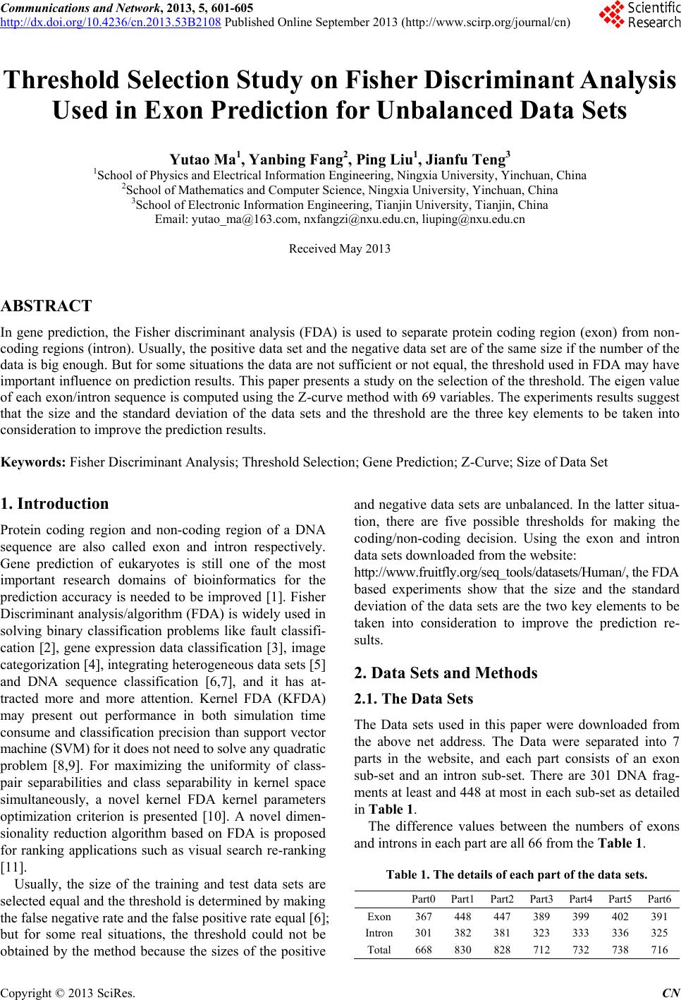