Intelligent Information Management, 2011, 3, 22-31
doi:10.4236/iim.2011.31003 Published Online January 2011 (http://www.SciRP.org/journal/iim)
Simulated Annealing Algorithm to Minimize Makespan
in Single Machine Scheduling Problem with
Uniform Parallel Machines
Panneerselvam Senthilkumar1, Sockalingam Narayanan2
1Program Management Office, Product Development, Mahindra & Mahindra Ltd. – Farm Division, Mumbai, India
2VIT University, Vellore, India
Received December 12, 2010; revised December 26, 2010; accepted January 5, 2011
Abstract
This paper presents a simulated annealing algorithm to minimize makespan of single machine scheduling
problem with uniform parallel machines. The single machine scheduling problem with uniform parallel ma-
chines consists of n jobs, each with single operation, which are to be scheduled on m parallel machines with
different speeds. Since, this scheduling problem is a combinatorial problem; usage of a heuristic is inevitable
to obtain the solution in polynomial time. In this paper, simulated annealing algorithm is presented. In the
first phase, a seed generation algorithm is given. Then, it is followed by three variations of the simulated an-
nealing algorithms and their comparison using ANOVA in terms of their solutions on makespan.
Keywords: Uniform Parallel Machines, Measure of Performance, Heuristic, Simulated Annealing Algorithm,
ANOVA
1. Introduction
The single machine scheduling problem is classified into
single machine scheduling with single machine and sin-
gle machine scheduling problem with parallel machines.
The single machine scheduling problem with single ma-
chine consists of n independent jobs, each with single
and same operations. The single machine scheduling
with parallel machines is further classified into the fol-
lowing three categories.
• Single machine scheduling with identical parallel
machines
• Single machine scheduling with uniform parallel
machines
• Single machine scheduling with unrelated parallel
machines
Let, tij be the processing times of the job j on the ma-
chine i, for i = 1, 2, 3,…., m and j = 1 2, 3,…, n.
Then the three types of parallel machines scheduling
problem are defined using this processing time.
1) If tij = t1j for all i and j, then the problem is called
as identical parallel machines scheduling problem.
This means that all the parallel machines are iden-
tical in terms of their speed. Each and every job
will take the same amount of processing time on
each of the parallel machines.
2) If tij = t1j/si for all i and j, where si is the speed of
the machine i and t1j is the processing time of the
job j on the machine 1, then the problem is termed
as uniform (proportional) parallel machines sche-
duling problem.
This means that the parallel machines will have
different speeds. Generally, we assume s1, s2, s3,….,
and sm for the parallel machines 1, 2, 3,…, and m,
respectively with the relation s1 < s2 < s3 < …. < sm.
That is the machine 1 is the slowest machine and
the machine m is the fastest machine. For a given
job, its processing times on the parallel machines
will be in the ratios as listed below.
1/s1 : 1/s2 : 1/s3 : …. : 1/sm
3) If tij is arbitrary for all i and j, then the problem is
known as unrelated parallel machines scheduling
problem.
In this type of scheduling, there will not be any re-
lation amongst the processing times of a job on the
parallel machines.
In this paper, the single machine scheduling problem
with uniform parallel machines is studied to minimize

P. SENTHILKUMAR ET AL. 23
the makespan. When n jobs with single operation are
scheduled on m parallel machines, then each parallel
machine will have its completion time of the last job in it.
The maximum of such completion times on all the paral-
lel machines is known as the makespan of the parallel
machines scheduling problem, which is an important
measure of performance, Panneerselvam [1].
The essential characteristics of the uniform parallel
machines scheduling problem are as listed below.
• It has n single operation jobs.
• It has m parallel machines with different speeds (s1
< s2 < s3 < ….. < sm).
• m machines are continuously available and they are
never kept idle while work is waiting
• t1j is the processing time of the job j on the ma-
chine 1 for j = 1, 2, 3,…, n.
• For each job, its processing times on the uniform
parallel machines are inversely proportional to the
speeds of those parallel machines (1/s1 : 1/s2 :
1/s3 : ….. : 1/sm), where s1 is the unit speed.
• tij = t1j/si for j = 1, 2, 3, …., n and i = 2, 3,….., m.
A sample data of the uniform parallel machines sched-
uling problem is shown in Table 1, in which the speed
ratio between the machine 1 and the machine 2 is 1 : 2.
In this paper, off-line, non-preemptive single machine
scheduling problem with uniform parallel machines is
considered.
To quote few practical examples of this uniform par-
allel machines scheduling problem, consider the machine
shop of an automobile company. Over a period of time,
machines of similar processing nature will be added to
enhance the capacity of the shop. The machines which
are added at the later stage will have higher speed when
compared to the old existing machines. One can establish
a speed ratio of the speeds of these two categories of
machines. If n independent single operation jobs are
scheduled on these two categories of machines collec-
tively to minimize the makespan, this practical reality
corresponds to single machine scheduling problem with
uniform parallel machines with the objective of mini-
mizing the makespan.
2. Review of Literature
In this section, the review of off-line, non-preemptive
Table 1. Processing times of jobs on uniform parallel ma-
chines.
Job j
Machine i Speed Ratio
1 2 3 4 5 6
1 1 1210 6 16 14 8
2 2 6 5 5 8 7 4
single machine scheduling problem with uniform parallel
machines is presented.
Horowitz and Sahni [2] first presented dynamic pro-
gramming algorithms for scheduling independent tasks
in a multiprocessor environment in which the processors
have different speeds. In this research, the objective is
minimize the finish time (makespan) and weighted mean
flow time on two processors. Next, they presented ap-
proximation algorithms of low polynomial complexity
for the above problem. Ibarra and Kim [3] have devel-
oped a heuristic for scheduling independent tasks on
nonidentical processors. In their study, particularly, for m
= 2, an nlogn time-bounded algorithm is given which
generates a schedule having a finishing time of at most


522 of the optimal finishing time. They verified
that the LPT algorithm applied to this problem gives
schedules which are near optimal for larger n. Prabuddha
De and Thomas E. Morton [4] have developed a new
heuristic to schedule jobs on uniform parallel processors
to minimize makespan. They found that the solutions
given by the heuristic for the uniform parallel machines
scheduling are within 5% of the solutions given by the
branch and bound algorithm. Bulfin and Parker [5] have
considered the problem of scheduling tasks on a system
consisting of two parallel processors such that the make-
span is minimized. In particular, they treated a variety of
modifications to this basic theme, including the cases of
identical processors, proportional (uniform) processors
and unrelated processors.
Friesen and Langston [6] examined the non-preemp-
tive assignment of n independent tasks to a system of m
uniform processors with the objective of reducing the
makespan. It is known that LPT (longest processing time
first) schedules are within twice the length of the opti-
mum makespan. Graham [7] analyzed a variation of the
MULTIFIT algorithm derived from the algorithm for bin
packing problem and proved that its worst-case per-
formance bound on the makespan is within 1.4 times of
the optimum makepsan. Gregory Dobson [8] has given a
worst-case analysis while applying the LPT (longest
processing Time) heuristic to the problem of scheduling
independent tasks on uniform processors with the mini-
mum makepsan. Friesen [9] examined the nonpreemptive
assignment of independent tasks to a system of uniform
processors with the objective of minimizing the make-
span. The author showed that the worst case bound for
the largest processing time first (LPT) algorithm for this
problem is tightened to be in the interval (1.52 to 1.67).
Hochbaum and Shmoys [10] devised a polynomial ap-
proximation scheme for the minimizing makespan prob-
lem on uniform parallel processors.
Chen [11] has examined the non-preemptive assign-
ment of independent tasks to a system of m uniform
processors with the objective of minimizing the makesp-

P. SENTHILKUMAR ET AL. 24
an. The author has examined the performance of LPT
(largest processing time) schedule with respect to opti-
mal schedules, using the ratio of the fastest speed to the
slowest speed of the system as a parameter.
Mireault, Orlin, Vohra [12] have considered the prob-
lem of minimizing the makespan when scheduling inde-
pendent tasks on two uniform parallel machines. Out of
the two machines, the efficiency of one machine is q
times as that of the other machine. They computed the
maximum relative error of the LPT (largest processing
time first) heuristic as a function of q. For the special
case in which the two machines are identical (q = 1),
their problem and heuristic are identical to the problem
and heuristic analyzed by Graham [7], respectively.
Burkard and He [13] derived the tight worst case bound

62 12k  for scheduling jobs using the MULTIFIT
heuristic on two parallel uniform machines with k calls
of FFD (first fit decreasing) within MULTIFIT .
Burkard, He and Kellerer [14] have developed a linear
compound algorithm for scheduling jobs on uniform par-
allel machines with the objective of minimizing makespan.
This algorithm has three subroutines, which run inde-
pendently in order to choose the best assignment among
them. Panneerselvam and Kanagalingam [15] have pre-
sented a mathematical model for parallel machines
scheduling problem with varying speeds in which the
objective is to minimize the makespan. Also, they dis-
cussed industrial applications of such scheduling prob-
lem. Panneerselvam and Kanagalingam [16] have given
a heuristic to minimize the makespan for scheduling n
independent jobs on m parallel processors with different
speeds.
Chandra Chekuri and Michael Bender [17] designed a
new and efficient polynomial 6 approximation algorithm
for scheduling precedence-constrained jobs on uniform
parallel machines. Chudak and Shmoys [18] gave an
algorithm with an approximation ratio of O (log m), sig-
nificantly improving the earlier ratio of O (m) due to
Jaffe [19]. Their algorithm is based on solving a linear
programming relaxation. Building on some of their ideas,
Chandra Chekuri and Michael Bender [20] have pre-
sented a combinatorial algorithm that achieves a similar
approximation ratio but in O (n3) time. Ching-Jong Liao
and Chien-Hung Lin [21] have considered the two uni-
form parallel machines problem with the objective of
minimizing makespan. In this work, the two uniform
parallel machines problem is converted into a special
problem of two identical parallel machines from the
viewpoint of workload instead of completion time. An
optimal algorithm is developed for the transformed spe-
cial problem. The proposed algorithm has an exponential
time complexity.
Christos Koulamas and George J. Kyparisis [22] in-
vestigated the makespan minimization problem on uni-
form parallel machines in the presence of release times.
They developed a heuristic for this NP-hard problem and
derived a tight worst-case ratio bound for this heuristic
independent of the machines speeds. Agarwal, Colak,
Jacob and Pirkul [23] have proposed new heuristics
along with an augmented-neural-netwrok (AugNN) for-
mulation for solving the makespan minimization task-
scheduling problem for the non-identical machine envi-
ronment. Chein-Hung Lin and Ching-Jong Liao [24]
have considered a classical scheduling problem with
makespan minimization on uniform parallel machines.
From the viewpoint of workload, instead of completion
time, two important theorems are developed for the
problem.
From the literature, it is clear that the objective of
minimizing the makespan in single machine scheduling
problem with uniform parallel machines comes under
combinatorial category. Hence, development of heuristic
is inevitable for this problem. Hence, a simulated an-
nealing algorithm is presented in this paper.
3. Simulated Annealing Algorithm
This section presents a simulated annealing algorithm to
minimize the makespan in the single machine scheduling
problem with uniform parallel machines. The simulated
annealing algorithm has emerged from annealing which
is a heat treatment process. Annealing aims to bring back
the metallurgical structure of components which are ei-
ther hammered/cold drawn, etc. This heat treatment
process is called annealing, which will release the inter-
nal stress and strain of the component, there by changing
the misaligned grain structure to its original grain struc-
ture. The above process of annealing is mapped to solve
optimization problems, especially combinatorial prob-
lems and it is termed as “simulated annealing algorithm”.
The parameters of the simulated annealing algorithm are
given as:
T – temperature
r – a range from 0 to 1 which is used to reduce the
temperature
δ – a small positive number provided by the user
The skeleton of the simulated annealing algorithm ap-
plied to minimization problem is given as follows.
Step 0: Input T, r and δ
Step 1: Get an initial feasible solution S0 and compute
the related value of the objective function f (S0).
Step 2: Get an initial temperature, T > 0.
Step 3: Generate feasible solution S1 in the neighbour-
hood of So and compute the related value of the objective
function f (S1).
Step 4: Compute d = f (S0) – f (S1).

P. SENTHILKUMAR ET AL. 25
Step 5: Update S0.
5.1. If d > 0, set S0 = S1 and go to Step 6; else go to
Step 5.2.
5.2. Generate uniformly distributed random number in
the range 0 to 1 (R).
5.3. If R < e(d/T),then set S0 = S1and go to Step 6; else
go to Step 6.
Step 6: Set T = r x T.
Step 7: If T > δ, then go to Step 3; otherwise go to
Step 8.
Step 8: Use local optimization to reach a local opti-
mum starting from the last S0 value.
Step 9: Stop
In simulated annealing, there are three schemes of per-
turbation as listed below.
1) Shifting a job from one machine to another ma-
chine.
2) Exchanging jobs between two machines.
3) Transferring a job from one of the existing ma-
chines to a new machine (This is an infeasible
scheme in this type of scheduling).
Under the third scheme, a new machine will have to be
included to accommodate the job which is transferred
from any of the existing machines. The given problem
has a fixed number of machines (m). Hence, the usage of
the third scheme of perturbation is not possible. From the
skeleton of the simulated annealing algorithm, it is clear
that for good solution, researcher should use an efficient
seed generation algorithm and it should be followed by
the second phase to obtain global optimum solution.
3.1. Seed Generation Algorithm
The steps of a seed generation algorithm used in the
simulated annealing algorithm are presented in this sec-
tion.
Step 1: Input the following.
• Number of independent jobs with single operation
(n)
• Number of uniform parallel machines (m) with
speeds s1, s2, s3,…, sm.
• Processing times of the jobs on the uniform parallel
machines.
• Previous maximum makespan (PMS), a very high
value (10^6).
Step 2: Rearrange the jobs as per their longest proc-
essing time order based on their processing times on the
machine 1 (decreasing order of processing time from left
to right).
Step 3: For each job Q in the longest processing time
order array, from left to right, perform the following.
3.1. Add the current job as the last job to each of the
machines and compute the temporary completion time of
that job on each machine.
3.2. Find the minimum (MIN) of the temporary com-
pletion times of that job on all the machines and
identify the corresponding machine number (P).
3.3. Update the following:
a) Completion time of the last job on the machine P
to MIN.
b) Increment the number of jobs assigned to the ma-
chine P by 1.
N(P) = N(P) + 1
c) Store the current job Q at the position N(P) on the
machine P as shown below.
JOBP,N(P) = Q
Step 4: Find the maximum of the completion times of
the last jobs on all the machines and treat it as the
makespan (MS) of the current schedule.
Let, the machine on which this maximum makespan
occurs be R.
Step 5: If MS ≥ PMS then go to Step 9; otherwise, up-
date PMS = MS and go to Step 6.
Interchanging the jobs between machines is starting
from machine R to Machine 1 if they yield reduction in
makespan.
Step 6: Set INDEX1 = 0 and INDEX2 = 0
Step 7: For each job (job at the position I) from left to
right on the machine R, perform the following.
7.1. Set I = 1
7.2. Store the immediate preceding machine (Slower
machine) number with respect to the machine R in S.
S = R – 1
7.3. If the completion time of the last job on the ma-
chine S is 0, then go to Step 7.5; otherwise, go to Step 7.4.
7.4. For each job (Job at the position J) in machine S
from left to right, perform the following.
7.4.1. Set J = 1
7.4.2. Temporarily exchange the Job at the position I
on the machine R with the Job at the position J on the
machine S and find the maximum of the completion
times of the last jobs on all the machines (MAX_MS).
7.4.3. If MAX_MS < MS, then exchange the job at the
position I on the machine R and the job at the position J
on the machine S and go to Step 7.4.4; otherwise, go to
Step 7.4.5.
7.4.4. Update PMS = MAX_MS.
7.4.5. Update INDEX1 = 1 and INDEX2 = 1
7.4.5. Increment the job position on the machine S by
1 (J = J + 1).
7.4.6. If J ≤ the last position on the machine S, then go
to Step 7.4.7; otherwise, go to Step 7.4.8.
7.4.7. If INDEX2 = 0 then go to Step 7.4.2; otherwise,
set INDEX2 = 0 and go to Step 7.4.1.
7.5. Decrement slower machine number (S) by 1 (S =
S – 1).

P. SENTHILKUMAR ET AL. 26
7.6. If S ≥ 1, then go to Step 7.3; otherwise, go to Step
8.
Step 8: If INDEX1 = 1, then go to Step 4; otherwise,
go to Step 9.
Step 9: Print the following results.
a) Assignment of jobs on the machines JOBi, j, i = 1, 2,
3,…., m and j = 1, 2, 3,…., N(i)
b) Makespan of the schedule, MS.
3.2. Simulated Annealing Algorithm to Minimize
Makespan
In this section, three different simulated annealing algo-
rithms (SA1, SA2 and SA3) are presented to minimize
the makespan in the single machine scheduling problem
with uniform parallel machines. The differences in these
algorithms are in terms of selection of the machines for
exchanging the jobs as well as transferring a job from
one machine to another machine. The details are shown
in Table 2. Through experimentation, the parameters of
the simulated annealing algorithm are set at: T = 60, r =
0.85 and δ = 0.01.
3.2.1. Simulated Annealing Algorithm SA1
The steps of the simulated annealing algorithm SA1 are
presented in this section. In this algorithm, while select-
ing two machines for exchanging jobs in them as well as
transferring a job from one machine to another machine,
they are selected with equal probability, which is equal
to 1/m, where m is the total number of uniform parallel
machines.
Step 1: Input the following.
• Number of independent jobs with single operation
(n)
• Number of uniform parallel machines (m) with
speeds s1, s2, s3,…, sm.
• Processing times of the jobs on the uniform parallel
machines.
Step 2: Obtain an initial feasible schedule (S0) using
the seed generation algorithm given in Subsection 3.1.
Let the corresponding makespan of the schedule of the
initial feasible solution be f (S0).
Step 3: Set T = 60, r = 0.85 and δ = 0.01.
Step 4: Generating feasible solution S1 in the neigh-
borhood of S0 and computing corresponding make- span,
f (S1).
4.1. Generate uniformly distributed random number, R
in between 0 to 0.99.
4.2. If R ≤ 0.49 then go to Step 4.3; else go to Step 4.4.
4.3. Exchange of jobs between two machines.
4.3.1. Randomly select a machine (P1), which is as-
signed with at least one job for transferring a job from
that machine.
Table 2. Distinctions among the sa algorithms applied to
minimize makespan.
Algorithm
Probability of selection of
machines for exchanging
jobs
Probability of selec-
tion of machines for
transferring a job
from one machine
to another machine
SA1 Equal Equal
SA2 Inverse of the speed of the
machine Equal
SA3 Inverse of the speed of the
machine
Inverse of the speed
of the machine
4.3.2. Randomly select a job from the machine P1 and
let it be Q1.
4.3.3. Randomly select another machine (P2), which is
assigned with at least one job for transferring a job from
that machine.
4.3.4. Randomly select a job from the machine P2 and
let it be Q2.
4.3.5. Exchange the jobs Q1 and Q2 between the ma-
chines P1 and P2.
4.3.6. Compute the makespan of this schedule, f(S1).
Go to Step 5.
4.4. Transfer of a job from one machine to another
machine.
4.4.1. Randomly select a machine (P1), which is as-
signed with at least one job for transferring a job from
that machine.
4.4.2. Randomly select a job from the machine P1 and
let it be Q1.
4.4.3. Randomly select another machine (P2) to which
the job Q1 is to be transferred.
4.4.4. Transfer the job Q1 from the machine P1 to the
machine P2.
4.4.5. Compute the makespan of this schedule, f(S1).
Go to Step 5.
Step 5. Compute d = f (S0) – f (S1).
Step 6. Updating S0.
6.1. If d > 0, set S0 = S1 and go to Step 7; else go to
Step 6.2.
6.2. Generate uniformly distributed random number (R)
in the range 0 to 1.
6.3. If R < e (d/T), then set S0 = S1 and go to Step 7;
else go to Step 7.
Step 7. Set T = r × T
Step 8. If T > δ, then go to Step 4; otherwise go to Step
9.
Step 9. Use the seed generation algorithm (local opti-
mum procedure) to reach a local optimum starting from
the last S0 value and print the final schedule.
Step 10: Stop.

P. SENTHILKUMAR ET AL. 27
3.2.2. Simulated Annealing Algorithm SA2
The steps of the simulated annealing algorithm SA2 are
presented in this section. In this algorithm, while select-
ing two machines for exchanging jobs, each ma- chine is
selected with a probability equal to the inverse of its speed
ratio. But, while transferring a job from one machine to
another machine, each machine is selected with equal
probability, which is equal to 1/m, where m is the total
number of uniform parallel machines.
Step 1: Input the following.
• Number of independent jobs with single operation
(n)
• Number of uniform parallel machines (m) with
speeds s1, s2, s3,…, sm.
• Processing times of the jobs on the uniform parallel
machines.
Step 2: Obtain an initial feasible schedule (S0) using
the seed generation algorithm given in Section 3.1. Let
the corresponding makespan of the schedule of the initial
feasible solution be f (S0).
Step 3: Set T = 60, r = 0.85 and δ = 0.01.
Step 4: Generating feasible solution S1 in the neighbor-
hood of S0 and computing corresponding makespan, f
(S1).
4.1. Generate uniformly distributed random number, R
in between 0 to 0.99.
4.2. If R ≤ 0.49 then go to Step 4.3; else go to Step 4.4.
4.3. Exchange of jobs between two machines.
4.3.1. Randomly select a machine (P1), which is as-
signed with at least one job for transferring a job from
that machine, by assuming inverse of the speed ratio as
the probability of selection for each of the machines.
4.3.2. Randomly select a job from the machine P1 and
let it be Q1.
4.3.3. Randomly select another machine (P2), which is
assigned with at least one job for transferring a job from
that machine, by assuming inverse of the speed ratio as
the probability of selection for each of the machines.
4.3.4. Randomly select a job from the machine P2 and
let it be Q2.
4.3.5. Exchange the jobs Q1 and Q2 between the ma-
chines P1 and P2.
4.3.6. Compute the makespan of this schedule, f(S1).
Go to Step 5.
4.4. Transfer of a job from one machine to another
machine.
4.4.1. Randomly select a machine (P1), which is as-
signed with at least one job for transferring a job from
that machine.
4.4.2. Randomly select a job from the machine P1 and
let it be Q1.
4.4.3. Randomly select another machine (P2) to which
the job Q1 is to be transferred.
4.4.4. Transfer the job Q1 from the machine P1 to the
machine P2.
4.4.5. Compute the makespan of this schedule, f(S1).
Go to Step 5.
Step 5: Compute d = f (S0) – f (S1).
Step 6: Updating So.
6.1. If d > 0, set So = S1 and go to Step 7; else go to
Step 6.2.
6.2. Generate uniformly distributed random number (R)
in the range 0 to 1.
6.3. If R < e(d/ T), then set So = S1 and go to Step 7;
else go to Step 7.
Step 7: Set T = r × T
Step 8: If T > δ, then go to Step 4; otherwise go to Step
9.
Step 9: Use the seed generation algorithm (local opti-
mum procedure) to reach a local optimum starting from
the last S0 value and print the final schedule.
Step 10: Stop.
3.2.3. Simulated Annealing Algorithm SA3
The steps of the simulated annealing algorithm SA3 are
presented in this section. In this algorithm, while select-
ing two machines for exchanging jobs as well as trans-
ferring a job from one machine to another machine, each
machine is selected with a probability equal to the in-
verse of its speed ratio.
Step 1: Input the following.
• Number of independent jobs with single operation
(n)
• Number of uniform parallel machines (m) with
speeds s1, s2, s3,…, sm.
• Processing times of the jobs on the uniform parallel
machines.
Step 2: Obtain an initial feasible schedule (S0) using
the seed generation algorithm given in Section 3.1. Let
the corresponding makespan of the schedule of the initial
feasible solution be f (S0).
Step 3: Set T = 60, r = 0.85 and δ = 0.01.
Step 4: Generating feasible solution S1 in the neigh-
borhood of S0 and computing corresponding makespan, f
(S1).
4.1. Generate uniformly distributed random number, R
in between 0 to 0.99.
4.2. If R ≤ 0.49 then go to Step 4.3; else go to Step 4.4.
4.3. Exchange of jobs between two machines.
4.3.1. Randomly select a machine (P1), which is as-
signed with at least one job for transferring a job from
that machine, by assuming inverse of the speed ratio as
the probability of selection for each of the machines.
4.3.2. Randomly select a job from the machine P1 and
let it be Q1.
4.3.3. Randomly select another machine (P2), which is

P. SENTHILKUMAR ET AL. 28
assigned with at least one job for transferring a job from
that machine, by assuming inverse of the speed ratio as
the probability of selection for each of the machines.
4.3.4. Randomly select a job from the machine P2 and
let it be Q2.
4.3.5. Exchange the jobs Q1 and Q2 between the ma-
chines P1 and P2.
4.3.6. Compute the makespan of this schedule, f(S1).
Go to Step 5.
4.4. Transfer of a job from one machine to another
machine.
4.4.1. Randomly select a machine (P1), which is as-
signed with at least one job for transferring a job from
that machine, by assuming inverse of the speed ratio as
the probability of selection for each of the machines.
4.4.2. Randomly select a job from the machine P1 and
let it be Q1.
4.4.3. Randomly select another machine (P2) to which
the job Q1 is to be transferred, by assuming inverse of
the speed ratio as the probability of selection for each of
the machines.
4.4.4. Transfer the job Q1 from the machine P1 to the
machine P2.
4.4.5. Compute the makespan of this schedule, f(S1).
Go to Step 5.
Step 5: Compute d = f (S0) – f (S1).
Step 6: Updating S0.
6.1. If d > 0, set S0 = S1 and go to Step 7; else go to
Step 6.2.
6.2. Generate uniformly distributed random number (R)
in the range 0 to 1.
6.3. If R < e (d/T), then set So = S1 and go to Step 7;
else go to Step 7.
Step 7: Set T = r × T
Step 8: If T > δ, then go to Step 4; otherwise go to
Step 9.
Step 9: Use the seed generation algorithm (local opti-
mum procedure) to reach a local optimum starting from
the last S0 value and print the final schedule.
Step 10: Stop.
4. Experimentation with the Algorithms
As stated earlier, in this paper, three simulated annealing
algorithms are presented. So, the next step is to compare
them in terms of their solutions. Hence, an experiment is
designed using randomized complete block design to
compare the algorithms. In this experiment, the number
of machines is varied form 2 to 4 and the number of jobs
is varied from 5 to 25. For each of the combinations of
the number of uniform parallel machines and the number
of jobs which are to be scheduled in them, data on proc-
essing times have been randomly generated by assuming
the speed ratio of 1 for the machine-1 and speed ration of
m for the machine-m. The results on makespan using the
algorithms are summarized in Table 3.
The model of the randomized complete block design
used to analyze the data shown in Table 3 is shown be-
low.
Yij = μ + Bi + Tj + eij
where, Yij is the makespan w. r. t. ith block (problem)
under the jth treatment of algorithm.
μ is the overall mean
Bi is the effect of the ith block (Problem) on the
makespan.
Tj is the effect of the jth algorithm on the makespan.
eij is the random error associated with the makespan w.
r. t. ith block(problem) and jth algorithm.
Factor: Algorithm
H0: There is no significant difference between the al-
gorithms (SA1, SA2 and SA3) in terms of the makespan.
H1: There is significant difference between the algo-
rithms (SA1, SA2 and SA3), for at least one pair of algo-
rithms in terms of the makespan.
Block: Problem
H0: There is no significant difference between the
problems in terms of makespan.
H1: There is significant difference between the prob-
lems, for at least one pair of the problems in terms of the
makespan.
The results of this ANOVA are summarized in Table
4.
Inference:
The calculated F ratio of the factor “Algorithm” is
0.0252 which is less than the table F ratio of 3, at a sig-
nificance level of 0.05. Hence, the null hypothesis w. r. t.
this factor is accepted. This means that there is no sig-
nificant difference between the algorithms in terms of the
makespan.
The calculated F ratio of the block “Problem” is
36199.49 which is more than the table F ratio of
1.319667, at a significance level of 0.05. Hence, the null
hypothesis w. r. t. this block is rejected. This means that
there is significant difference between problems in terms
of the makespan.
Since, it is proved that there is no significant differ-
ence between the algorithms, it is suggested to use each
of the three algorithms (SA1, SA2 and SA3) for a given
problem and select the best result. As per this suggestion,
the results shown in Table 3 are analyzed as shown in
Table 5. From Table 5, it is seen that the percentage
number of best solutions for the algorithms SA1, SA2
and SA3 are 77.78%, 87.3, and 77.78%, respectively. If
the best of the results of the three algorithms is selected
as the solution for each problem, the percentage number
of best solutions is 100%.
From the analysis, it is clear that solving a given problem

P. SENTHILKUMAR ET AL. 29
Table 3. Results on makespan of the problems using three
algorithms.
Algorithm
Problem Size
SA1 SA2 SA3
2 × 5 100.5 100.5 100.5
2 × 6 102.0 96.0 102.0
2 × 7 93.0 93.0. 93.0
2 × 8 135.0 135.0 135.0
2 × 9 181.5 184.0 181.5
2 × 10 183.0 183.5 183.0
2 × 11 199.0 199.0 199.0
2 × 12 203.0 204.5 203.0
2 × 13 255.0 255.0 255.0
2 × 14 222.0 223.0 222.0
2 × 15 337.5 338.5 337.5
2 × 16 284.5 285.5 284.5
2 × 17 330.5 330.5 330.5
2 × 18 376.0 376.0 376.0
2 × 19 321.0 319.5 321.0
2 × 20 302.0 308.0 302.0
2 × 21 409.0 406.0 409.0
2 × 22 408.0 408.0 408.0
2 × 23 398.5 404.0 398.5
2 × 24 361.0 361.0 361.0
2 × 25 467.5 464.0 467.5
3 × 5 48.0 48.0 48.0
3 × 6 64.5 66.3 64.5
3 × 7 58.7 58.6 58.7
3 × 8 84.0 83.6 84.0
3 × 9 87.0 86.0 87.0
3 × 10 106.7 106.7 106.7
3 × 11 86.0 86.0 86.0
3 × 12 122.0 122.0 122.0
3 × 13 121.7 122.0 121.7
3 × 14 122.5 122.5 122.5
3 × 15 146.0 143.0 146.0
3 × 16 152.3 152.0 152.3
3 × 17 168.5 167.0 168.5
3 × 18 152.0 152.0 152.0
3 × 19 194.3 193.0 194.3
3 × 20 189.0 189.0 189.0
3 × 21 212.3 212.0 212.3
3 × 22 218.0 213.6 218.0
3 × 23 224.0 224.0 224.0
3 × 24 215.0 215.0 215.0
3 × 25 212.0 212.0 212.0
4 × 5 25.0 25.0 25.0
4 × 6 39.3 39.3 39.3
4 × 7 43.8 43.8 43.8
4 × 8 57.5 57.5 57.5
4 × 9 46.5 46.5 46.5
4 × 10 54.3 56.5 54.3
4 × 11 59.3 59.3 59.3
4 × 12 75.0 74.8 75.0
4 × 13 69.0 69.0 69.0
4 × 14 76.8 76.8 76.8
4 × 15 87.3 87.3 87.3
4 × 16 84.3 84.3 84.3
4 × 17 93.0 93.0 93.0
4 × 18 111.0 111.0 111.0
4 × 19 107.0 107.0 107.0
4 × 20 105.5 105.5 105.5
4 × 21 127.5 127.5 127.5
4 × 22 120.5 121.6 120.5
4 × 23 135.0 135.0 135.0
4 × 24 143.0 143.0 143.
4 × 25 149.3 149.3 149.3
using all the three algorithms and then selecting the best
of the results of these algorithms as the solution for the
problem is more effective, when compared to the indi-
vidual usage of the three algorithms.
5. Conclusions
The objective of minimizing the makespan in single
machine scheduling problem with uniform parallel ma-
chines is a combinatorial problem. Hence, in this paper, a
simulated annealing approach is presented. In the first
phase, a seed generation algorithm is presented. In the
second phase, three different seed generation algorithms
(SA1, SA2 and SA3) are presented. An ANOVA using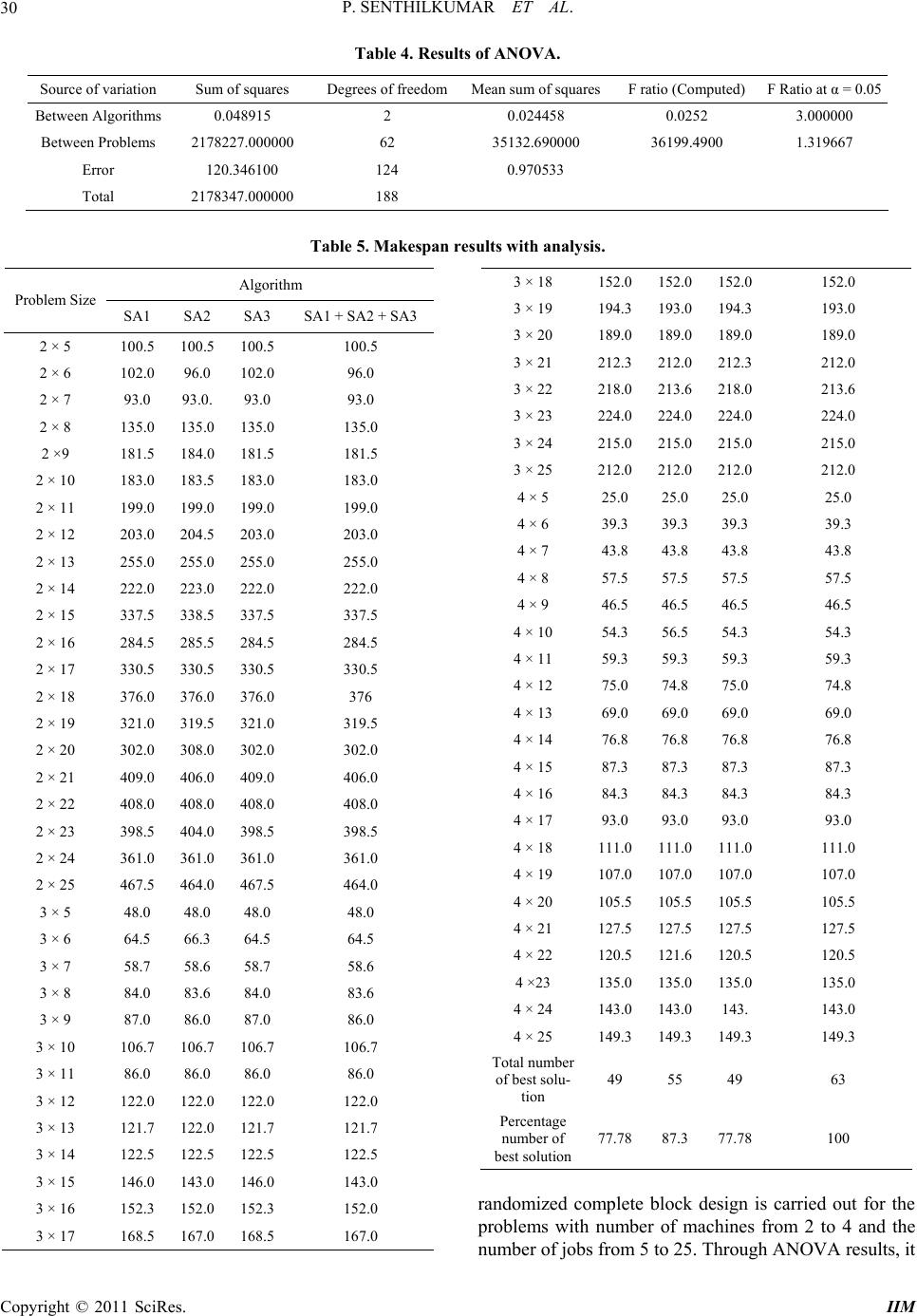

P. SENTHILKUMAR ET AL. 30
Table 4. Results of ANOVA.
Source of variation Sum of squares Degrees of freedomMean sum of squaresF ratio (Computed) F Ratio at α = 0.05
Between Algorithms 0.048915 2 0.024458 0.0252 3.000000
Between Problems 2178227.000000 62 35132.690000 36199.4900 1.319667
Error 120.346100 124 0.970533
Total 2178347.000000 188
Table 5. Makespan results with analysis.
Algorithm
Problem Size
SA1 SA2 SA3 SA1 + SA2 + SA3
2 × 5 100.5 100.5 100.5 100.5
2 × 6 102.0 96.0 102.0 96.0
2 × 7 93.0 93.0. 93.0 93.0
2 × 8 135.0 135.0 135.0 135.0
2 ×9 181.5 184.0 181.5 181.5
2 × 10 183.0 183.5 183.0 183.0
2 × 11 199.0 199.0 199.0 199.0
2 × 12 203.0 204.5 203.0 203.0
2 × 13 255.0 255.0 255.0 255.0
2 × 14 222.0 223.0 222.0 222.0
2 × 15 337.5 338.5 337.5 337.5
2 × 16 284.5 285.5 284.5 284.5
2 × 17 330.5 330.5 330.5 330.5
2 × 18 376.0 376.0 376.0 376
2 × 19 321.0 319.5 321.0 319.5
2 × 20 302.0 308.0 302.0 302.0
2 × 21 409.0 406.0 409.0 406.0
2 × 22 408.0 408.0 408.0 408.0
2 × 23 398.5 404.0 398.5 398.5
2 × 24 361.0 361.0 361.0 361.0
2 × 25 467.5 464.0 467.5 464.0
3 × 5 48.0 48.0 48.0 48.0
3 × 6 64.5 66.3 64.5 64.5
3 × 7 58.7 58.6 58.7 58.6
3 × 8 84.0 83.6 84.0 83.6
3 × 9 87.0 86.0 87.0 86.0
3 × 10 106.7 106.7 106.7 106.7
3 × 11 86.0 86.0 86.0 86.0
3 × 12 122.0 122.0 122.0 122.0
3 × 13 121.7 122.0 121.7 121.7
3 × 14 122.5 122.5 122.5 122.5
3 × 15 146.0 143.0 146.0 143.0
3 × 16 152.3 152.0 152.3 152.0
3 × 17 168.5 167.0 168.5 167.0
3 × 18 152.0152.0 152.0 152.0
3 × 19 194.3193.0 194.3 193.0
3 × 20 189.0189.0 189.0 189.0
3 × 21 212.3212.0 212.3 212.0
3 × 22 218.0213.6 218.0 213.6
3 × 23 224.0224.0 224.0 224.0
3 × 24 215.0215.0 215.0 215.0
3 × 25 212.0212.0 212.0 212.0
4 × 5 25.0 25.0 25.0 25.0
4 × 6 39.3 39.3 39.3 39.3
4 × 7 43.8 43.8 43.8 43.8
4 × 8 57.5 57.5 57.5 57.5
4 × 9 46.5 46.5 46.5 46.5
4 × 10 54.3 56.5 54.3 54.3
4 × 11 59.3 59.3 59.3 59.3
4 × 12 75.0 74.8 75.0 74.8
4 × 13 69.0 69.0 69.0 69.0
4 × 14 76.8 76.8 76.8 76.8
4 × 15 87.3 87.3 87.3 87.3
4 × 16 84.3 84.3 84.3 84.3
4 × 17 93.0 93.0 93.0 93.0
4 × 18 111.0111.0 111.0 111.0
4 × 19 107.0107.0 107.0 107.0
4 × 20 105.5105.5 105.5 105.5
4 × 21 127.5127.5 127.5 127.5
4 × 22 120.5121.6 120.5 120.5
4 ×23 135.0135.0 135.0 135.0
4 × 24 143.0143.0 143. 143.0
4 × 25 149.3149.3 149.3 149.3
Total number
of best solu-
tion
49 55 49 63
Percentage
number of
best solution
77.78 87.3 77.78 100
randomized complete block design is carried out for the
problems with number of machines from 2 to 4 and the
number of jobs from 5 to 25. Through ANOVA results, it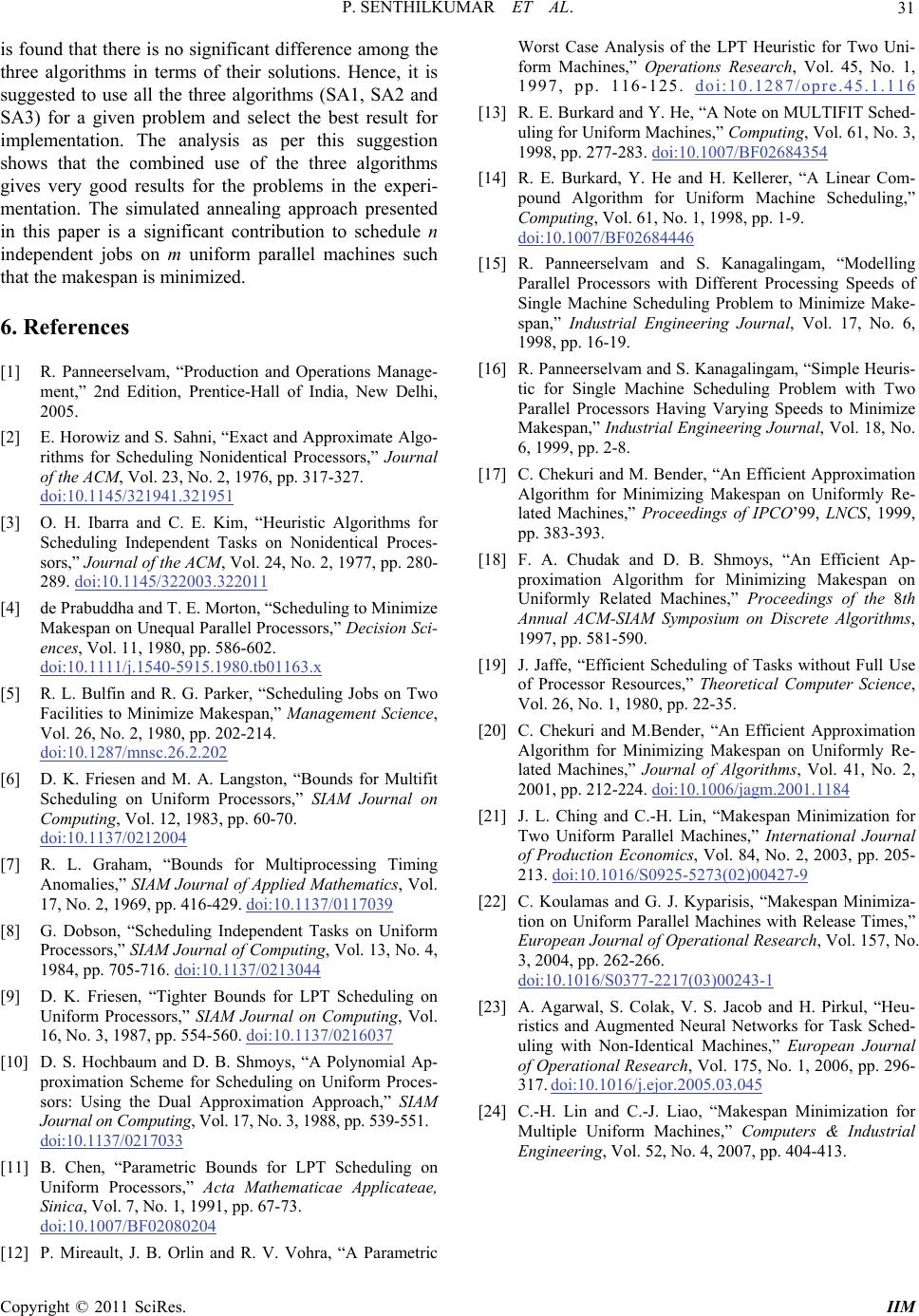

P. SENTHILKUMAR ET AL. 31
is found that there is no significant difference among the
three algorithms in terms of their solutions. Hence, it is
suggested to use all the three algorithms (SA1, SA2 and
SA3) for a given problem and select the best result for
implementation. The analysis as per this suggestion
shows that the combined use of the three algorithms
gives very good results for the problems in the experi-
mentation. The simulated annealing approach presented
in this paper is a significant contribution to schedule n
independent jobs on m uniform parallel machines such
that the makespan is minimized.
6. References
[1] R. Panneerselvam, “Production and Operations Manage-
ment,” 2nd Edition, Prentice-Hall of India, New Delhi,
2005.
[2] E. Horowiz and S. Sahni, “Exact and Approximate Algo-
rithms for Scheduling Nonidentical Processors,” Journal
of the ACM, Vol. 23, No. 2, 1976, pp. 317-327.
doi:10.1145/321941.321951
[3] O. H. Ibarra and C. E. Kim, “Heuristic Algorithms for
Scheduling Independent Tasks on Nonidentical Proces-
sors,” Journal of the ACM, Vol. 24, No. 2, 1977, pp. 280-
289. doi:10.1145/322003.322011
[4] de Prabuddha and T. E. Morton, “Scheduling to Minimize
Makespan on Unequal Parallel Processors,” Decision Sci-
ences, Vol. 11, 1980, pp. 586-602.
doi:10.1111/j.1540-5915.1980.tb01163.x
[5] R. L. Bulfin and R. G. Parker, “Scheduling Jobs on Two
Facilities to Minimize Makespan,” Management Science,
Vol. 26, No. 2, 1980, pp. 202-214.
doi:10.1287/mnsc.26.2.202
[6] D. K. Friesen and M. A. Langston, “Bounds for Multifit
Scheduling on Uniform Processors,” SIAM Journal on
Computing, Vol. 12, 1983, pp. 60-70.
doi:10.1137/0212004
[7] R. L. Graham, “Bounds for Multiprocessing Timing
Anomalies,” SIAM Journal of Applied Mathematics, Vol.
17, No. 2, 1969, pp. 416-429. doi:10.1137/0117039
[8] G. Dobson, “Scheduling Independent Tasks on Uniform
Processors,” SIAM Journal of Computing, Vol. 13, No. 4,
1984, pp. 705-716. doi:10.1137/0213044
[9] D. K. Friesen, “Tighter Bounds for LPT Scheduling on
Uniform Processors,” SIAM Journal on Computing, Vol.
16, No. 3, 1987, pp. 554-560. doi:10.1137/0216037
[10] D. S. Hochbaum and D. B. Shmoys, “A Polynomial Ap-
proximation Scheme for Scheduling on Uniform Proces-
sors: Using the Dual Approximation Approach,” SIAM
Journal on Computing, Vol. 17, No. 3, 1988, pp. 539-551.
doi:10.1137/0217033
[11] B. Chen, “Parametric Bounds for LPT Scheduling on
Uniform Processors,” Acta Mathematicae Applicateae,
Sinica, Vol. 7, No. 1, 1991, pp. 67-73.
doi:10.1007/BF02080204
[12] P. Mireault, J. B. Orlin and R. V. Vohra, “A Parametric
Worst Case Analysis of the LPT Heuristic for Two Uni-
form Machines,” Operations Research, Vol. 45, No. 1,
1997, pp. 116-125. doi:10.1287/opre.45.1.116
[13] R. E. Burkard and Y. He, “A Note on MULTIFIT Sched-
uling for Uniform Machines,” Computing, Vol. 61, No. 3,
1998, pp. 277-283. doi:10.1007/BF02684354
[14] R. E. Burkard, Y. He and H. Kellerer, “A Linear Com-
pound Algorithm for Uniform Machine Scheduling,”
Computing, Vol. 61, No. 1, 1998, pp. 1-9.
doi:10.1007/BF02684446
[15] R. Panneerselvam and S. Kanagalingam, “Modelling
Parallel Processors with Different Processing Speeds of
Single Machine Scheduling Problem to Minimize Make-
span,” Industrial Engineering Journal, Vol. 17, No. 6,
1998, pp. 16-19.
[16] R. Panneerselvam and S. Kanagalingam, “Simple Heuris-
tic for Single Machine Scheduling Problem with Two
Parallel Processors Having Varying Speeds to Minimize
Makespan,” Industrial Engineering Journal, Vol. 18, No.
6, 1999, pp. 2-8.
[17] C. Chekuri and M. Bender, “An Efficient Approximation
Algorithm for Minimizing Makespan on Uniformly Re-
lated Machines,” Proceedings of IPCO’99, LNCS , 1999,
pp. 383-393.
[18] F. A. Chudak and D. B. Shmoys, “An Efficient Ap-
proximation Algorithm for Minimizing Makespan on
Uniformly Related Machines,” Proceedings of the 8th
Annual ACM-SIAM Symposium on Discrete Algorithms,
1997, pp. 581-590.
[19] J. Jaffe, “Efficient Scheduling of Tasks without Full Use
of Processor Resources,” Theoretical Computer Science,
Vol. 26, No. 1, 1980, pp. 22-35.
[20] C. Chekuri and M.Bender, “An Efficient Approximation
Algorithm for Minimizing Makespan on Uniformly Re-
lated Machines,” Journal of Algorithms, Vol. 41, No. 2,
2001, pp. 212-224. doi:10.1006/jagm.2001.1184
[21] J. L. Ching and C.-H. Lin, “Makespan Minimization for
Two Uniform Parallel Machines,” International Journal
of Production Economics, Vol. 84, No. 2, 2003, pp. 205-
213. doi:10.1016/S0925-5273(02)00427-9
[22] C. Koulamas and G. J. Kyparisis, “Makespan Minimiza-
tion on Uniform Parallel Machines with Release Times,”
European Journal of Operational Research, Vol. 157, No.
3, 2004, pp. 262-266.
doi:10.1016/S0377-2217(03)00243-1
[23] A. Agarwal, S. Colak, V. S. Jacob and H. Pirkul, “Heu-
ristics and Augmented Neural Networks for Task Sched-
uling with Non-Identical Machines,” European Journal
of Operational Research, Vol. 175, No. 1, 2006, pp. 296-
317. doi:10.1016/j.ejor.2005.03.045
[24] C.-H. Lin and C.-J. Liao, “Makespan Minimization for
Multiple Uniform Machines,” Computers & Industrial
Engineering, Vol. 52, No. 4, 2007, pp. 404-413.