Applied Mathematics, 2013, 4, 17-25
http://dx.doi.org/10.4236/am.2013.410A1004 Published Online October 2013 (http://www.scirp.org/journal/am)
High-Precision Numerical Scheme for Vortical Flow
Kei Ito1*, Tomoaki Kunugi2, Hiroyuki Ohshima1
1Advanced Nuclear System Research and Development Directorate, Japan Atomic Energy Agency, Ibaraki, Japan
2Department of Nuclear Engineering, Kyoto University, Kyoto, Japan
Received June 10, 2013; revised July 10, 2013; accepted July 17, 2013
Copyright © 2013 Kei Ito et al. This is an open access article distributed under the Creative Commons Attribution License, which
permits unrestricted use, distribution, and reproduction in any medium, provided the original work is properly cited.
ABSTRACT
In this study, a new high-precision numerical simulation scheme for vortical flows (vortex-based scheme) is proposed.
This scheme identifies a vortical flow in each computational cell, and then, reconstructs a vortical velocity distribution
based on the Burgers vortex model. In addition, a pressure distribution in the vicinity of the vortex center is also re-
constructed. The momentum transfer is calculated with the reconstructed velocity and pressure distributions, and there-
fore, the vortex-based scheme can simulate vortical flows more accurately than the conventional schemes. In fact, as the
simulation result of inviscid vortex attenuation problem, the vortex-based scheme shows lower simulation error com-
pared to the conventional discretization schemes. Moreover, also in the numerical simulation of the quasi-steady vorti-
cal flow, the simulation accuracy of the vortex-based scheme is superior to those of the conventional schemes.
Keywords: Computational Fluid Dynamics; Numerical Scheme; Vortex Cavitation; Burgers Vortex Theory
1. Introduction
Vortex cavitation can be observed in various engineering
scenes, e.g. pump sump. However, in usual, the occur-
rence of the vortex cavitation is not favorable because the
vibration of structural components and/or the noise can
be induced by the vortex cavitation. Moreover, the cavi-
tation bubbles generated at the vortex core may damage a
structural surface when they collapse. Also in sodium-
cooled fast reactors [1], the sub-surface vortex cavitation
might be induced by high-speed suction flow into an out-
let pipe in the reactor vessel. However, the onset condi-
tion of the vortex cavitation cannot be clarified easily be-
cause the vortex cavitation shows highly complicated be-
haviors associated with phase change. Therefore, the au-
thors have conducted experimental and numerical studies
to evaluate the onset condition of the vortex cavitation.
As the experimental study, a fundamental experiment is
conducted to investigate the influence of the dynamic vi-
scosity on the onset condition [2], and some scale model
tests are also conducted to check the dependency on the
local structural geometry and the effect of countermea-
sure obstacles [3]. On the other hand, in the numerical
study, a high-precision simulation algorithm for sub-sur-
face vortex flows is under development, in which a un-
structured mesh scheme is employed to model accurately
the local structural geometry near a sub-surface vortex.
The high-precision numerical simulation algorithm is
developed originally for the evaluation of gas entrain-
ment phenomena in sodium-cooled fast reactors [4-6].
Currently, it is confirmed this algorithm can simulate the
gas entrainment phenomena caused by free surface vor-
tices, that is, dynamic vortex behaviors, i.e. vortex deve-
lopment, movement and attenuation, can be simulated.
Therefore, the algorithm is considered to be applicable to
numerical simulations of the vortex cavitation. However,
the numerical simulation of the vortex cavitation is not
easy because the sub-surface vortex has highly thin vor-
tex core compared to the free surface vortex. In other
words, it is very difficult to reproduce the velocity distri-
bution at the vicinity of the core of the sub-surface vortex.
In this case, a very fine mesh at the vicinity of the vortex
core and/or a high-precision numerical simulation scheme
should be employed to simulate the sub-surface vortex
accurately. A very fine mesh is easy to be constructed but
requires high computational cost which may exceeds the
limit of usable computational resource. Therefore, a high-
precision numerical simulation scheme is necessary to si-
mulate the sub-surface vortex accurately. Here, it should
be noted the implementation of well-known high order
(more than 2nd order) schemes, e.g. K-K scheme [7] are
difficult on unstructured meshes because of irregular com-
putational cell arrangement.
*Corresponding author.
C
opyright © 2013 SciRes. AM

K. ITO ET AL. 18
In this paper, a high-precision simulation scheme for
vortical flows on unstructured meshes is presented. In
conventional schemes, the velocity distribution between
computational cells is interpolated with the constant, li-
near or higher order functions based on the discrete val-
ues defined at the cells, and therefore, the existence of a
vortical flow is considered indirectly through the veloc-
ity distribution around the vortex. On the other hand, in
our new high-precision scheme, a vortical flow is identi-
fied in each cell and the vortical velocity distribution at
the vicinity of the vortex center is reconstructed locally
based on the Burgers vortex theory [8]. Namely, the ex-
istence of a vortical flow is considered directly in the
new high-precision scheme. In this sense, this new scheme
is called “the vortex-based scheme” in this paper. In ad-
dition to the velocity distribution, the pressure distribu-
tion at the vicinity of the vortex center is also considered
based on the Burgers vortex theory to simulate accurately
the mechanical balance between pressure gradient and
centrifugal force. Then, the calculations of momentum
transport through cell faces are performed in considera-
tion of the reconstructed velocity and pressure distribu-
tions. The superiority of the vortex-based scheme to the
conventional schemes is confirmed by the fundamental
verifications, such as the numerical simulation of vortex
attenuation.
2. Formulation of High-Precision Numerical
Scheme for Vortical Flow (Vortex-Based
Scheme)
2.1. The Identification of a Vortical Flow in Each
Computational Cell
In the vortex-based scheme, the existence of a vortical
flow is considered directly. Therefore, in the first place
of the calculation, vortical flows are identified by apply-
ing the discriminant [9,10] to each computational cell.
Namely, a vortex center exists in a cell when the follow-
ing discriminant is satisfied in the cell.
32
427DQ R 0, (1)
where Q and R are the second and third invariants of the
velocity gradient tensor


,iji j
Au

 defined in each
cell.
3
,1
ij ji
ij
QA

A, (2)
detRA, (3)
In the cell with a vortex center, the direction of the
vortex, i.e. the direction of the rotational axis, is obtained
as the eigen vector of the eigenvalue equation of the ve-
locity gradient tensor. Then, a plane is defined, which is
normal to the direction of the vortex center and passes
through the cell center. On this plane, the point with zero
in-plane velocity is determined as the vortex center.
2.2. The Supplement of the Vortical Velocity
Distribution
A strong vortical flow has very large velocity gradient in
the immediate vicinity of the vortex center. Therefore, it
is highly difficult to simulate such a velocity distribution
accurately with limited computer resources (lack of suf-
ficient number of cells). In the vortex-based scheme, the
vortical velocity distribution is supplemented in the vi-
cinity of the vortex center by utilizing the Burgers vortex
model which is known as an excellent model of the vor-
tices in nature, e.g. free surface vortices, sub-surface vor-
tices or turbulent vortices.
The circumferential velocity

u

distribution of the
Burgers vortex model is written as

2
0
1exp r ur rr








 
  







, (4)
where r is the radial coordinate with the origin at the
vortex center. Equation (4) has two parameters, i.e. the
circulation Γ and the specific radius r0. In the vortex-
based scheme, these parameters are determined to make
the circumferential velocity distribution consistent with
the local velocity distribution. Namely, upon a given (si-
mulated) velocity field, two parameters are adjusted to
minimize the difference in the circumferential velocity
distributions of Equation (4) and the given field at the
cells in the vicinity of a vortex center. The calculation pro-
cedure is shown in Figure 1 as follows:
1) a cell with a vortex center (called “vortex cell” in
this paper) is selected;
2) vertices on the vortex cell and the cells around the
vortex cell is selected;
3) when the velocity is given at the cell centers, the
circumferential velocities at the vertices

v
u

are inter-
polated from the cell center velocities

c
u

as follows:
surround
surround
cc
v
c
wu
uw




, (5)
where the summations are operated on all cells surroun-
ding each selected vertex, and wc is the weighting factor
for the summation;
4) the differences between the Burgers model (Equa-
tion (4)) and the circumferential velocities at the selected
vertices


v
u

 are calculated and averaged as the form
of the weighted root mean square (shown by an overbar)
as follows:

2
vertices
vv
uwu

 v

 , (6)

K. ITO ET AL. 19
Vortex
center
Vortex
cell
(a) (b) (c)
v
u


Burgers
(d) (e)
Figure 1. Procedure to determine vortex parameters: (a) selection of a vortex cell; (b) listing up of vertices; (c) interpolation
of circumferential velocity at each vertex (red vectors); (d) calculation of differences at each vertex (Burgers vortex velocity
in horizontal is shown by blue curve) and (e) adjustments of parameters.
where the summation is operated on all selected vertices,
and wv is the weighting factor for the summation;
5) the circulation and the specific radius are adjusted
iteratively to minimize the averaged differences


v
u

 .
The weighting factor in Equation (5) is determined by
minimizing the cost-function (Co in Equation (7)) under
the constraint formulated as Equation (8) [11], and the
weighting factor in Equation (6) is determined in a si-
milar manner.



2
surround
1
c
cv
Co w
r
in the numerical simulations on unstructured meshes. In
he cell based FVM is employed on an unstruc-
tu
, (7)
surround
0
ccv
w
r (8)
where cv is the vector joining a cell center to a vertex.
In Figure 1, the calculation procedure on a two-dimen-
sional structured mesh is shown for simplification. How-
ever, the calculation on a three-dimensional unstructured
mesh can be conducted in the same procedure.
r
2.3. The Momentum Transport Calculation
The finite volume method (FVM) is employed frequently
that case, each cell is generally selected as the control vo-
lumes for discretization. Also in our high-precision nu-
merical simulation algorithm, such simulation method
(cell based FVM) is employed, and therefore, the fol-
lowing description is given based on the cell based FVM.
However, the concept of the vortex-based scheme is ap-
plicable also to other methods, e.g. the finite difference
method.
When t
red mesh, it is difficult to formulate high order momen-
tum transport schemes, i.e. third or higher order schemes,
due to the irregular cell arrangement. Therefore, the first
and second order upwind schemes are used frequently for
the momentum transport calculation. In the first order up-
wind scheme, the momentum on a cell face is determined
to be same as that in the upwind cell of the cell face. On
the other hand, in the second order upwind scheme,
the momentum on a cell face

f
m is calculated in
consideration of the momentum ( and momentum
c
m)
gradient



c
m in the upwincell of the cell d
(9)
face:

c
fc cf
mm mr,

K. ITO ET AL. 20
where is the vector joining the upwi
cf
r
fac
nd cell center to
the celle center. In Equation (9), the momentum gra-
dient can be calculated by the Gauss-Green method [11]
or Least-square method [12]. The first or second order
upwind scheme works well in the numerical simulations
of smooth flows without discontinuity (shock) and strong
vortices. However, as mentioned briefly in Section 2.2,
the velocity distribution in the vicinity of a vortex center
is very sharp and a very high resolution mesh is neces-
sary to simulate the vortical velocity distribution accu-
rately by the first or second order upwind scheme. Instead
of such a very high resolution mesh, which is not appli-
cable to practical simulations, the vortex-based scheme
supplements the vortical velocity distribution in the vi-
cinity of a vortex center by the Burgers vortex model
(Equation (4)) and calculates the momentum transport
based on the supplemented velocity distribution. Namely,
when the velocity distribution in the vicinity of a vortex
center is given by Equation (4), the momentum in the cir-
cumferential direction

f
m

is calculated on a cell face
as
f
ff
mu


 , (10)
where
f

is the fluid density on the cell face and
f
u

is the cmferential velocity at the cell face center c
culated by Equation (4). Then, the momentum transport
is calculated based on Equation (10).
2.4. The Pressure Calculation
ircu al-
In the vicinity of a vortex center, not only the velocity
gradient but also the pressure gradient is large due to the
mechanical balance between the circumferential velocity
and the pressure gradient (see Equation (11)). Therefore,
the pressure should be supplemented to simulate vortical
flows accurately. In the vortex-based scheme, the pres-
sure distribution in the vicinity of a vortex center is cal-
culated in consideration of the mechanical balance equa-
tion of the circumferential velocity and the pressure gra-
dient, written as
2
up
rr


, (11)
where p is the pressure. Substituting the circumferential
velocity distribution of the Burges model (Equation (4))
into Equation (11) leads the pressure distribution.
 


2
2
2
3
0
1exp d
R
R
pRR R
rR
  






, (12)
where 0
Rrr

. The pressure calculated by Equation
(12) is applied to the faces on a vortex cell and the faces
on the cells around the vortex cell. Then, the pressure
gradient term in the momentum transport equation (Na-
vier-Stokes equation) is calculated at each cell based on
the applied pressure values.
3. Verification
3.1. The Reproducibility of a Vortical Flow
As the first verification, the reproducibility of a vortex by
the vortex-based scheme is addressed. In this calculation,
the Burgers vortex is set on two-dimensional structured
meshes, and then, the identification and the velocity sup-
plement calculations are conducted to check the repro-
ducibility of the vortex. As shown in Figure 2, the simu-
lation domain is 1.00 × 1.00 and subdivided into 8 × 8
square cells. The velocity distribution of the Burgers vor-
tex is applied to all cells with various vortex center posi-
tions, specific radii and/or circulation values.
Table 1 shows the calculation results. It is evident that
the vortex center position and the circulation are well re-
Table 1. Reproducibility of Burgers vortex.
Original (given) valuesvalues Calculated
Vortex center coordinSpecific radiusVortex center coordinate Specific radius ate Circulation Circulation
(0.00, 0.00) 0.100 0.050 (0.00, 0.00) 0.106 0.107
0.100 0.102 0.138
0.125 0.102 0.158
0.200 0.101 0.221
0.250 0.100 0.267
(0.01,.00) (0.0094,.0005)
0.
1.00 (0.00, 0.00) 1.00 0.267
0 00.100 0.267
(0.01, 0.01) (0.0103, 0.0098) 0.100 0.267
(0.05, 0.05) (0.0503, 0.0488) 0.100 0.266
(0.00, 0.00) 010 (0.00, 0.00) 0.010 0.267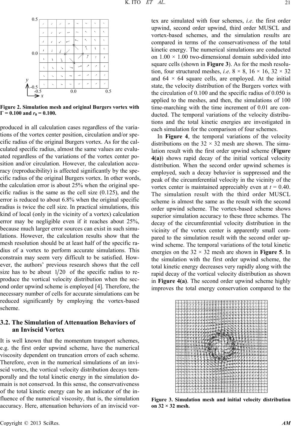

K. ITO ET AL. 21
x
y
-0.5 0.0 0.5
0.5
0.0
-0.5
Figure 2. Simulation mesh and original Burgers vortex with
Γ = 0.100 and r0 = 0.100.
r position, circulation and/or spe-
ific radius of the original Burgers vortex. As for the cal-
produced in all calculation cases regardless of the varia-
tions of the vortex cente
c
culated specific radius, almost the same values are evalu-
ated regardless of the variations of the vortex center po-
sition and/or circulation. However, the calculation accu-
racy (reproducibility) is affected significantly by the spe-
cific radius of the original Burgers vortex. In other words,
the calculation error is about 25% when the original spe-
cific radius is the same as the cell size (0.125), and the
error is reduced to about 6.8% when the original specific
radius is twice the cell size. In practical simulations, this
kind of local (only in the vicinity of a vortex) calculation
error may be negligible even if it reaches about 25%,
because much larger error sources can exist in such simu-
lations. However, the calculation results show that the
mesh resolution should be at least half of the specific ra-
dius of a vortex to perform accurate simulations. This
constrain may seem very difficult to be satisfied. How-
ever, the authors’ previous research shows that the cell
size has to be about 120 of the specific radius to re-
produce the vortical velocity distribution when the sec-
ond order upwind scheme is employed [4]. Therefore, the
necessary number of cells for accurate simulations can be
reduced significantly by employing the vortex-based
scheme.
3.2. The Simulation of Attenuation Behaviors of
an Inviscid Vortex
,
viscosity deation errors of each scheme.
tex ted with foures, i.e. the first order
upwd order upwiird order M and
vortex-bschemes, and thulation
the
pe
It is well known that the momentum transport schemes
e.g. the first order upwind scheme, have the numerical
pendent on trunc
Therefore, even in the numerical simulations of an invi-
scid vortex, the vortical velocity distribution decays tem-
porally and the total kinetic energy in the simulation do-
main is not conserved. In this sense, the conservativeness
of the total kinetic energy can be an indicator of the in-
fluence of the numerical viscosity, that is, the simulation
accuracy. Here, attenuation behaviors of an inviscid vor-
compared in terms of the conservativeness of the total
kinetic energy. The numerical simulations are conducted
on 1.00 × 1.00 two-dimensional domain subdivided into
square cells (shown in Figure 3). As for the mesh resolu-
tion, four structured meshes, i.e. 8 × 8, 16 × 16, 32 × 32
and 64 × 64 square cells, are employed. At the initial
state, the velocity distribution of the Burgers vortex with
the circulation of 0.100 and the specific radius of 0.050 is
applied to the meshes, and then, the simulations of 100
time-marching with the time increment of 0.01 are con-
ducted. The temporal variations of the velocity distribu-
tions and the total kinetic energies are investigated in
each simulation for the comparison of four schemes.
In Figure 4, the temporal variations of the velocity
distributions on the 32 × 32 mesh are shown. The simu-
lation result with the first order upwind scheme (Figure
4(a)) shows rapid decay of the initial vortical velocity
distribution. When the second order upwind schemes is
employed, such a decay behavior is suppressed and
are simula schem
ind, secon
ased
nd, th
e sim
USCL
results are
ak of the circumferential velocity in the vicinity of the
vortex center is maintained appreciably even at t = 0.40.
The simulation result with the third order MUSCL
scheme is almost the same as the result with the second
order upwind scheme. The vortex-based scheme shows
superior simulation accuracy to these three schemes. The
decay of the circumferential velocity distribution in the
vicinity of the vortex center is apparently small com-
pared to the simulation result with the second order up-
wind scheme. The temporal variations of the total kinetic
energies on the 32 × 32 mesh are shown in Figure 5. In
the simulation with the first order upwind scheme, the
total kinetic energy decreases very rapidly along with the
rapid decay of the vortical velocity distribution as shown
in Figure 4(a). The second order upwind scheme highly
improves the total energy conservation compared to the
Figure 3. Simulation mesh and initial velocity distribution
on 32 × 32 mesh.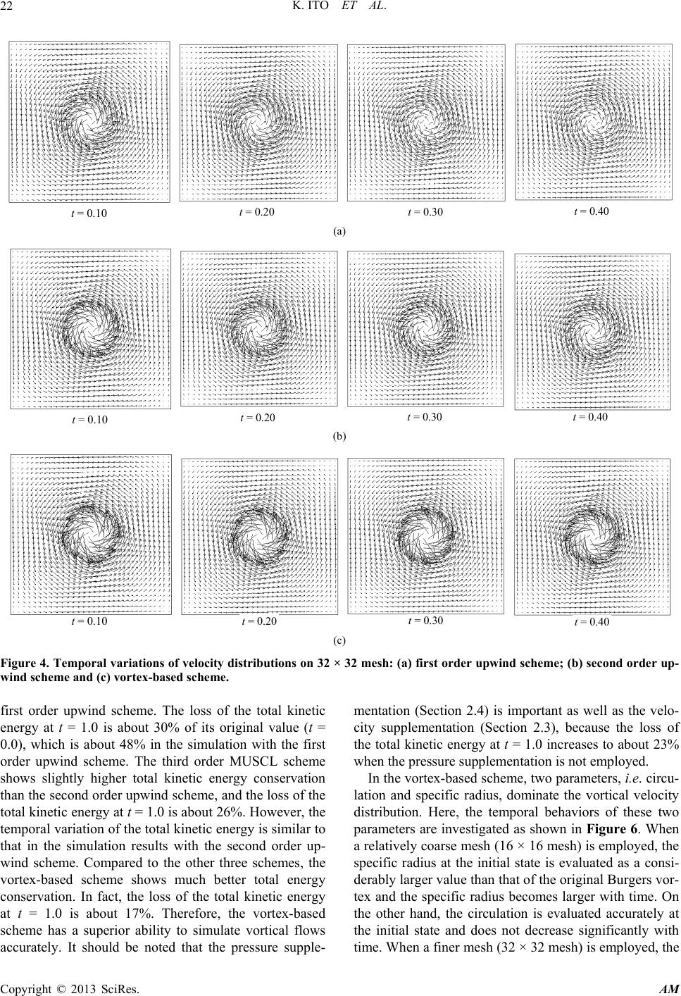

K. ITO ET AL. 22
t
= 0.10
t = 0.20
t = 0.30
t = 0.40
(a)
t
= 0.10
t = 0.20 t = 0.30
t = 0.40
(b)
t = 0.10 t = 0.20
t = 0.30
t = 0.40
(c)
Figure 4. Temporal variations of velocity distributions on 32 × 32 mesh: (a) first order upwind scheme; (b) second order up-
wind scheme and (c) vortex-based scheme.
first order upwind scheme. The loss of the total kinetic
energy at t = 1.0 is about 30% of its original value (t =
0.0), which is about 48% in the simulation with the first
order upwind scheme. The third order MUSCL scheme
shows slightly higher total kinetic energy conservation
than the second order upwind scheme, and the loss of the
total kinetic energy at t = 1.0 is about 26%. However, the
temporal variation of the total kinetic energy is similar to
that in the simulation results with the second order up-
wind scheme. Compared to the other three schemes, the
l kinetic energy
t t = 1.0 is about 17%. Therefore, the vortex-based
mentation (Section 2.4) is important as well as the velo-
city supplementation (Section 2.3), because the loss of
the total kinetic energy at t = 1.0 increases to about 23%
when the pressure supplementation is not employed.
In the vortex-based scheme, two parameters, i.e. circu-
lation and specific radius, dominate the vortical velocity
distribution. Here, the temporal behaviors of these two
parameters are investigated as shown in Figure 6. When
a relatively coarse mesh (16 × 16 mesh) is employed, th
specific radius at the initial state is evaluated as a consi-
tex and the specific radius becomes larger with time. On
the other hand, the circulation is evaluated accurately at
vortex-based scheme shows much better total energy
conservation. In fact, the loss of the tota
derably larger value than that of the original Burgers vor-
a
scheme has a superior ability to simulate vortical flows
accurately. It should be noted that the pressure supple-
the initial state and does not decrease significantly with
time. When a finer mesh (32 × 32 mesh) is employed, the
e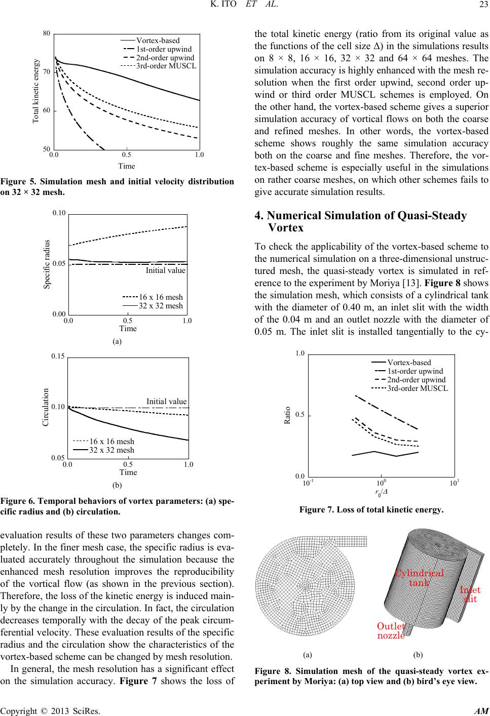

K. ITO ET AL. 23
50
60
70
80
0.0 0.5 1.0
Vortex-based
1st-order upwind
2nd-order upwind
3rd-order MUSCL
Total kinetic energy
Time
Figure 5. Simulation mesh and initial velocity distribution
on 32 × 32 mesh.
0.00
0.05
0.10
0.0 0.5 1.0
16 x 16 mesh
32 x 32 mesh
Specific radius
Time
Initial value
(a)
0.05
0.10
0.15
0.0 0.5 1.0
16 x 16 mesh
32 x 32 mesh
Circulation
Time
Initial value
(b)
) circulation.
evaluation results of these two parameters changes com-
pletely. In the finer mesh case, the specific radius is eva-
luated accurately throughout the simulation because the
enhanced mesh resolution improves the reproducibility
of the vortical flow (as shown in the previous section).
Therefore, the loss of the kinetic energy is induced main-
ly by the change in the circulation. In fact, the circulation
decreases temporally with the decay of the peak circum-
ferential velocity. These evaluation results of the specific
radius and the circulation show the characteristics of the
vortex-based scheme can banged by mesh resolution.
In general, the mesh resolution has a significant effect
on the simulation accuracy. Figure 7 shows the loss of
the total kinetic energy (ratio from its original value as
the functions of the cell size Δ) in the simulations results
on 8 × 8, 16 × 16, 32 × 32 and 64 × 64 meshes. The
simulation accuracy is highly enhanced with the mesh re-
solution when the first order upwind, second order up-
wind or third order MUSCL schemes is employed. On
the other hand, the vortex-based scheme gives a superior
simulation accuracy of vortical flows on both the coarse
and refined meshes. In other words, the vortex-based
scheme shows roughly the same simulation accuracy
both on the coarse and fineshes. Thereforhe vor-
tex-based scheme is especi useful in the simulations
s.
Figure 6. Temporal behaviors of vortex parameters: (a) spe-
cific radius and (b
e ch
e m
ally
e, t
on rather coarse meshes, on which other schemes fails to
ive accurate simulation resultg
4. Numerical Simulation of Quasi-Steady
Vortex
To check the applicability of the vortex-based scheme to
the numerical simulation on a three-dimensional unstruc-
tured mesh, the quasi-steady vortex is simulated in ref-
erence to the experiment by Moriya [13]. Figure 8 shows
the simulation mesh, which consists of a cylindrical tank
with the diameter of 0.40 m, an inlet slit with the width
of the 0.04 m and an outlet nozzle with the diameter of
0.05 m. The inlet slit is installed tangentially to the cy-
0.0
0.5
1.0
10-1 100101
Vortex-bas ed
1st-order upwind
2nd-order upwind
3rd-order MUSCL
Ratio
r0/ 
Figure 7. Loss of total kinetic energy.
Inlet
slit
Outlet
nozzle
tank
(a) (b)
Figure 8. Simulation mesh of the quasi-steady vortex ex-
Cylindrical
eriment by Moriya: (a) top view and (b) bird’s eye view. p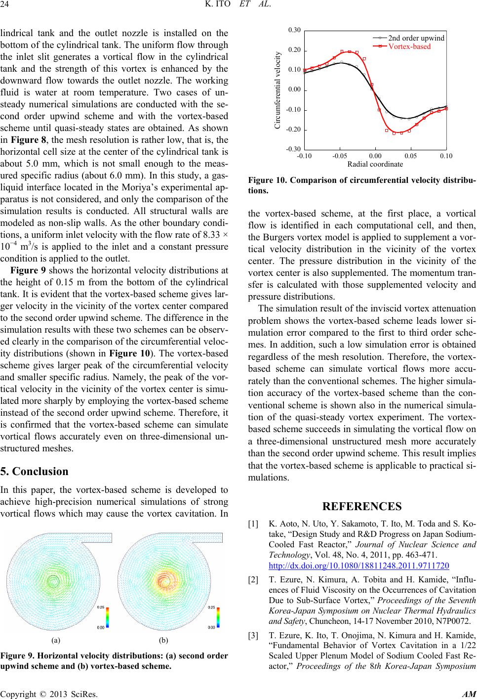

K. ITO ET AL. 24
lindrical tank and the outlet nozzle is installed on the
bottom of the cylindrical tank. The uniform flow through
the inlet slit generates a vortical flow in the cylindrical
tank and the strength of this vortex is enhanced by the
downward flow towards the outlet nozzle. The working
fluid is water at room temperature. Two cases of un-
steady numerical simulations are conducted with the se-
cond order upwind scheme and with the vortex-based
scheme until quasi-steady states are obtained. As shown
in Figure 8, the mesh resolution is rather low, that is, the
horizontal cell size at the center of the cylindrical tank is
about 5.0 mm, which is not small enough to the meas-
ured specifi gas-
quid inteental ap-
aratus is not considered, and only the comparison of the
simulation results is conducted. All structural walls are
modeled as non-slip walls. As the other boundary condi-
tions, a uniform inlet velocity with8.33 ×
10−4 m
3/s is applied to the inlet a pressure
condition is applied to the outlet.
Figure 9 shows the horizontal velocity distributt
the height of 0.15 m from the bottom of the cylindrical
tank. It is evident that the vor scheme gives lar-
ger velocity in the vicinity ofcenter compared
to the seconfference in th
simulation can be observ-
c radius (about 6.0 mm). In this study
rface located in the Moriya’s experim
, a
li
p
the flow rate of
nd a constant
ions a
tex-based
the vortex
d order upwindcheme. The di
results with these two schemes
se
ed clearly in the comparison of the circumferential veloc-
ity distributions (shown in Figure 10). The vortex-based
scheme gives larger peak of the circumferential velocity
and smaller specific radius. Namely, the peak of the vor-
tical velocity in the vicinity of the vortex center is simu-
lated more sharply by employing the vortex-based scheme
instead of the second order upwind scheme. Therefore, it
is confirmed that the vortex-based scheme can simulate
vortical flows accurately even on three-dimensional un-
structured meshes.
5. Conclusion
In this paper, the vortex-based scheme is developed to
achieve high-precision numerical simulations of strong
vortical flows which may cause the vortex cavitation. In
(a) (b)
Figure 9. Horizontal velocity distributions: (a) second order
upwind scheme and (b) vortex-based scheme.
-0.30
-0.20
-0.10
0.00
0.10
0.20
0.30
-0.10
2nd order upwind
Vortex-based
Circumferential velocity
-0.050.00 0.05 0.10
Radial coordinate
flow is identified in each computational cell, and then,
the Burgers vortex model is applied to supplement a vor-
tical velocity distribution in the vicinity of the vortex
center. The pressure distribution in the vicinity of the
vortex center is also supplemented. The momentum tran-
sfer is calculated with those supplemented velocity and
pressure distributions.
The simulation result of the inviscid vortex attenuation
problem shows the vortex-based scheme leads lower si
mulation errd order sche-
the vortex-
based scheme can simulate vortical flows more accu-
rately than the conventional schemes. The higher simula-
tion accuracy of the vortex-based scheme than the con-
ventional scheme is shown also in the numerical simula-
tion of the quasi-steady vortex experiment. The vortex-
based scheme succeeds in simulating the vortical flow on
a three-dimensional unstructured mesh more accurately
than the second order upwind scheme. This result implies
that the vortex-based scheme is applicable to practical si-
mulations.
REFERENCES
y and R&D Progress on Japan Sodium-
Figure 10. Comparison of circumferential velocity distribu-
tions.
the vortex-based scheme, at the first place, a vortical
-
or compared to the first to thir
mes. In addition, such a low simulation error is obtained
regardless of the mesh resolution. Therefore,
[1] K. Aoto, N. Uto, Y. Sakamoto, T. Ito, M. Toda and S. Ko-
take, “Design Stud
Cooled Fast Reactor,” Journal of Nuclear Science and
Technology, Vol. 48, No. 4, 2011, pp. 463-471.
http://dx.doi.org/10.1080/18811248.2011.9711720
[2] T. Ezure, N. Kimura, A. Tobita and H. Kamide, “Influ-
ences of Fluid Viscosity on the Occurrences of Cavitation
Due to Sub-Surface Vortex,” Proceedings of the Seventh
Korea-Japan Symposium on Nuclear Thermal Hydraulics
and Safety, Chuncheon, 14-17 November 2010, N7P0072.
[3] T. Ezure, K. Ito, T. Onojima, N. Kimura and H. Kamide,
“Fundamental Behavior of Vortex Cavitation in a 1/22
Scaled Upper Plenum Model of Sodium Cooled Fast Re-
actor,” Proceedings of the 8th Korea-Japan Symposium

K. ITO ET AL. 25
on Nuclear Thermal Hydraulics and Safety, Beppu, 9-12
December 2012, N8P1068.
[4] K. Ito, T. Kunugi, H. Ohshima and T. Kawamura, “Formu-
lations and Validations of a High-Precision Volume-of-
Fluid Algorithm on Non-Orthogonal Meshes for Nume-
rical Simulations of Gas Entrainment Phenomena,” Jour-
nal of Nuclear Science and Technology, Vol. 46, No. 4,
2009, pp. 366-373.
http://dx.doi.org/10.1080/18811248.2007.9711542
[5] K. Ito, T. Kunugi and H. Ohshima, “High-Precision Re-
construction of Gas-Liquid Interface in PLIC-VOF
Framework on Unstructured Mesh,” In: A. Kuzumin, Ed.,
Computational Fluid Dynamics 2010, Springer, Berlin,
2011, pp. 563-567.
http://dx.doi.org/10.1007/978-3-642-17884-9_71
[6] K. Ito, T. Kunugi and H. Ohshima, “A High-Precision
Unstructured ue for Gas-Liquid Adaptive Mesh Techniq
Two-Phase Flows,” International Journal for Numerical
Methods in Fluids, Vol. 67, No. 11, 2011, pp. 1571-1589.
http://dx.doi.org/10.1002/fld.2432
[7] T. Kawamura, H. Takami and K. Kuwahara, “Computa-
tion of High Reynolds Number Flow around a C
Cylinder with Surface Roughness,” Fluid Dynamiircular cs Re-
search, Vol. 1, No. 2, 1986, pp. 145-162.
http://dx.doi.org/10.1016/0169-5983(86)90014-6
[8] J. M. Burgers, “A Mathematical Model Illustrating the
Theory of Turbulence,” In: R. Mises and T. Karman, Eds.,
Advance in Applied Mechanics, Academic Press ING.,
New York, 1982, pp. 171-199
[9] K. Sawada, “A Convenient Visualization Method f
.
or Iden-
eport AIAA-95-1715,
tifying Vortex Center,” Transaction of the Japan Society
for Aeronautical and Space Sciences, Vol. 38, No. 120,
1995, pp. 102-116.
[10] D. Sujudi and R. Haimes, “Identification of Swirling Flow
in 3-D Vector Fields,” Technical R
American Institute of Aeronautics and Astronautics, 1995.
[11] D. Kim and H. Choi, “A Second-Order Time-Accurate
Finite Volume Method for Unsteady Incompressible Flow
on Hybrid Unstructured Grids,” Journal of Computatio-
nal Physics, Vol. 162, No. 2, 2000, pp. 411-428.
http://dx.doi.org/10.1006/jcph.2000.6546
[12] T. J. Barth and D. C. Jespersen, “The Design and Appli-
cation of Upwind Schemes on Unstructured Meshes,”
Technical Report AIAA-89-0366, AIAA 27th Aerospace
odel Test Measurements,” Technical
Sciences Meeting, Reno, 9-12 January 1989.
[13] S. Moriya, “Estimation of Hydraulic Characteristics of
Free Surface Vortices on the Basis on Extension Vortex
Theory and Fine M
Reports of Central Research Institute of Electric Power
Industry U97072, 1998.
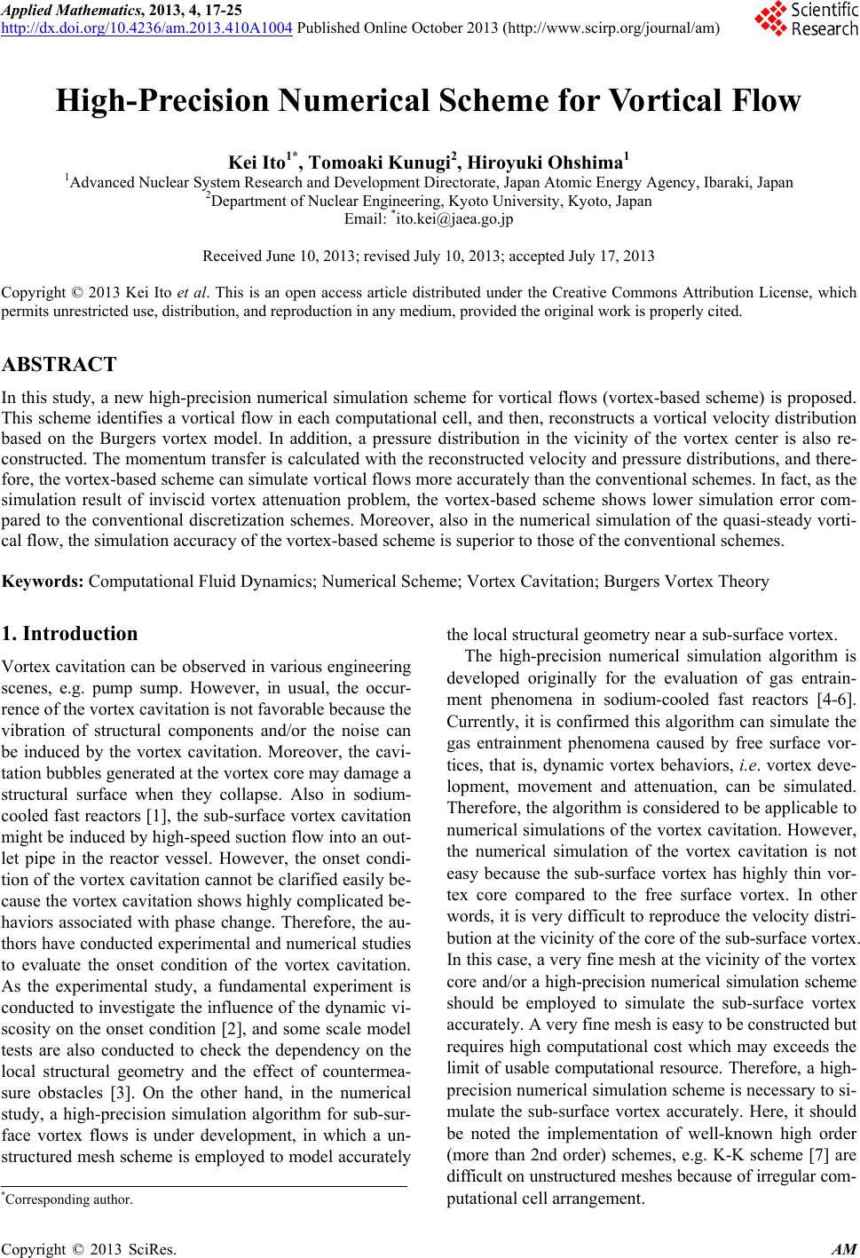