Open Journal of Applied Sciences, 2013, 3, 323-331
http://dx.doi.org/10.4236/ojapps.2013.35042 Published Online September 2013 (http://www.scirp.org/journal/ojapps)
Comparing the Effects of Interactive and Noninteractive
Complementary Nutrients on Growth in a Chemostat
James P. Braselton, Martha L. Abell, Lorraine M. Braselton
Department of Mathematical Sciences, Georgia Southern University, Statesboro, USA
Received July 12, 2013; revised August 12, 2012; accepted August 19, 2013
Copyright © 2013 James P. Braselton et al. This is an open access article distributed under the Creative Commons Attribution Li-
cense, which permits unrestricted use, distribution, and reproduction in any medium, provided the original work is properly cited.
ABSTRACT
We compare the effects of interactive and noninteractive complementary nutrients on the growth of an organism in the
chemostat. We also compare these two situations to the case when the nutrients are substitutable. In previous studies,
complementary nutrients have been assumed to be noninteractive. However, more recent research indicates that some
complementary nutrient relationships are interactive. We show that interactive complementary and substitutable nutri-
ents can lead to higher population densities than do noninteractive complementary nutrients. We numerically illustrate
that if the washout rate is high, an organism can persist at higher densities when the complementary nutrients are inter-
active than when they are noninteractive, which can result in the extinction of the organism. Finally, we present an ex-
ample by making a small adjustment to the model that leads to a single nutrient model with an intermediate metabolite
of the original substrate as the nutrient for the organism.
Keywords: Chemostat; Growth; Dual Substrate; Complementary Nutrients; Substitutable Nutrients
1. Introduction
We consider a basic, resource-based model of growth in
the chemostat. Such models have applications in ecology
to model a simple lake and in biotechnology to model the
commercial bio-reactor. Experimental verification of the
match between theory and experiment in the chemostat
can be found in [1]. Basic growth in the chemostat is
described by the dimensionless system


 
  
0
d,0 0
d
d,0 0.
d
S
Sx
SSD fSS
ty
xfS Dxx
t

 
(1)
For a detailed discussion of growth in the chemostat
and a description of the constants (input of the
nutrient), yS (yield constant), and D (dilution (washout)
rate), see Smith and Waltman [2].

0
S
Two nutrients are complementary if they meet differ-
ent needs for an organism. For example, ammonia pro-
vides nitrogen while glucose provides carbon [3] (build-
ing blocks of protein). Similarly, two nutrients are sub-
stitutable if they meet the same needs for an organism.
For example, glucose, galactose, maltose, ribose, arabi-
nose, and fructose all provide energy (sugar) [4].
See Stroot et al. [5], for a recent study of Acinetobac-
ter spp. bacteria in an activated sludge bioreactor system
using the noninteractive Monod model for multiple nu-
trients.
However, other research [3,4,6-9] indicates that a
model of interactive multiple limiting nutrients may be
more appropriate for some situations. Of particular inter-
est, Lendenmann and Egli [4] discuss several growth
models appropriate for substitutable interactive nutrients
and compare them to the growth of E. coli with sugar
nutrients glucose, galactose, maltose, ribose, arabinose,
and fructose. Whang et al. [9] perform a similar study
using bacteria from the wastewater of a food-processing
plant. On the other hand, Bapat et al. [10] use a Monod
model to study the growth of A. mediterranei S699 with
multiple interactive complementary nutrients. Champa-
gne et al. [11] form a model of cometabolism with two
interactive complementary nutrients in a well-mixed sys-
tem. Bae and Rittmann [12] develop a dual-limiting mo-
del, compare the results to experimental data, and ob-
serve that they agree, which provides further evidence
that a multiple nutrient limiting model might be more
appropriate in some situations than a single nutrient lim-
iting model. From [12], having an accurate kinetic model
for dual limitation is essential for a proper design of
treatment operations such as in bioremediation or con-
taminated groundwater... Dual limitation also can be
C
opyright © 2013 SciRes. OJAppS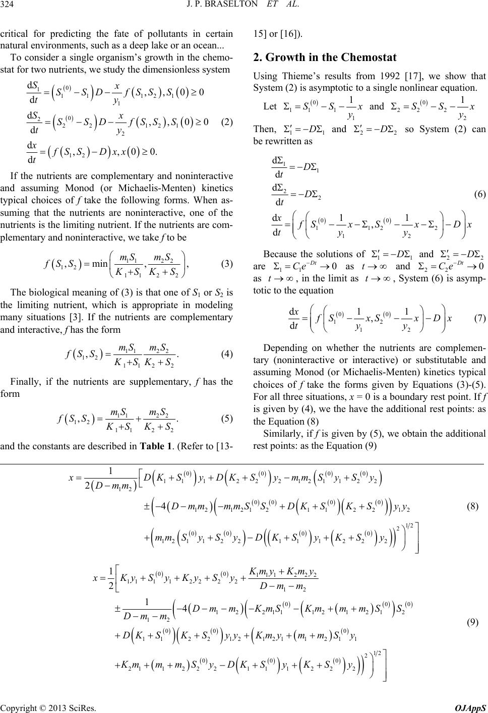

J. P. BRASELTON ET AL. 324
critical for predicting the fate of pollutants in certain
natural environments, such as a deep lake or an ocean...
To consider a single organism’s growth in the chemo-
stat for two nutrients, we study the dimensionless system






  
0
1
11 121
1
0
2
22 121
2
12
d,,00
d
d,,00
d
d,,00.
d
Sx
SSD fSSS
ty
Sx
SSDfSSS
ty
xfSS Dxx
t
 
 

(2)
If the nutrients are complementary and noninteractive
and assuming Monod (or Michaelis-Menten) kinetics
typical choices of f take the following forms. When as-
suming that the nutrients are noninteractive, one of the
nutrients is the limiting nutrient. If the nutrients are com-
plementary and noninteractive, we take f to be

112 2
12
11 22
,min ,
mSm S
fSS KSK S




, (3)
The biological meaning of (3) is that one of S1 or S2 is
the limiting nutrient, which is appropriate in modeling
many situations [3]. If the nutrients are complementary
and interactive, f has the form

112 2
12
112 2
,
mS mS
fSS .
K
SK S

(4)
Finally, if the nutrients are supplementary, f has the
form

112 2
12
112 2
,
mSm S
fSS .
K
SKS


(5)
and the constants are described in Table 1. (Refer to [13-
15] or [16]).
2. Growth in the Chemostat
Using Thieme’s results from 1992 [17], we show that
System (2) is asymptotic to a single nonlinear equation.
Let

0
11 1
1
1
SS
y
x
and

0
22 2
2
1
SS
y
x
Then, 11
D


 and 2 D2


 so System (2) can
be rewritten as
 
1
1
2
2
00
112 2
12
d
d
d
d
d11
,
d
D
t
D
t
x
f
SxS x D
ty y
 
 








x
(6)
Because the solutions of and
11
D

 22 D



are 11 0
Dt
Ce



t
as and 22
as , in the limit as , System (6) is asymp-
totic to the equation
t
t
0
Dt
Ce

 
00
12
12
d11
,
d
x
f
SxSxD
tyy


 





x
(7)
Depending on whether the nutrients are complemen-
tary (noninteractive or interactive) or substitutable and
assuming Monod (or Michaelis-Menten) kinetics typical
choices of f take the forms given by Equations (3)-(5).
For all three situations, x = 0 is a boundary rest point. If f
is given by (4), we the have the additional rest points: as
the Equation (8)
Similarly, if f is given by (5), we obtain the additional
rest points: as the Equation (9)






 






 

 




 

0000
1112 22121122
12
000 0
12121 2112212
12
2
000 0
12 1122111222
1
2
4
xDKSyDKSymmSySy
Dmm
DmmmmS SDKSKSyy
mm SySyD KSyKSy




 


 




(8)
 
















 



 
00
1112 22
11112 222
12
00
12211121212
12
00 0
1122121211211
12
2
000
2112 22111222
1
2
14
KmyKm y
xKySyKySyDm m
Dm mKmSKmmmSS
Dm m
DKSKSyyKmymmSy
KmmmSyDKSyKSy









 



0
(9)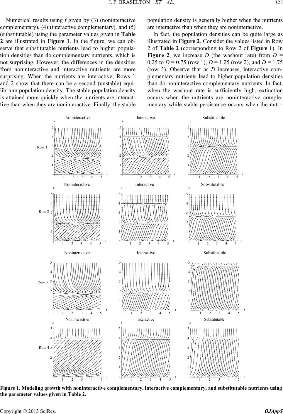

J. P. BRASELTON ET AL. 325
Numerical results using f given by (3) (noninteractive
complementary), (4) (interactive complementary), and (5)
(substitutable) using the parameter values given in Table
2 are illustrated in Figure 1. In the figure, we can ob-
serve that substitutable nutrients lead to higher popula-
tion densities than do complementary nutrients, which is
not surprising. However, the differences in the densities
from noninteractive and interactive nutrients are more
surprising. When the nutrients are interactive, Rows 1
and 2 show that there can be a second (unstable) equi-
librium population density. The stable population density
is attained more quickly when the nutrients are interact-
tive than when they are noninteractive. Finally, the stable
population density is generally higher when the nutrients
are interactive than when they are noninteractive.
In fact, the population densities can be quite large as
illustrated in Figur e 2. Consider the values listed in Row
2 of Tab l e 2 (corresponding to Row 2 of Figure 1). In
Figure 2, we increase D (the washout rate) from D =
0.25 to D = 0.75 (row 1), D = 1.25 (row 2), and D = 1.75
(row 3). Observe that as D increases, interactive com-
plementary nutrients lead to higher population densities
than do noninteractive complementary nutrients. In fact,
when the washout rate is sufficiently high, extinction
occurs when the nutrients are noninteractive comple-
mentary while stable persistence occurs when the nutri-
Row 1
Row 2
Row 3
Row 4
Figure 1. Modeling growth with noninteractive complementary, interactive complementary, and substitutable nutrients using
the parameter values given in Table 2.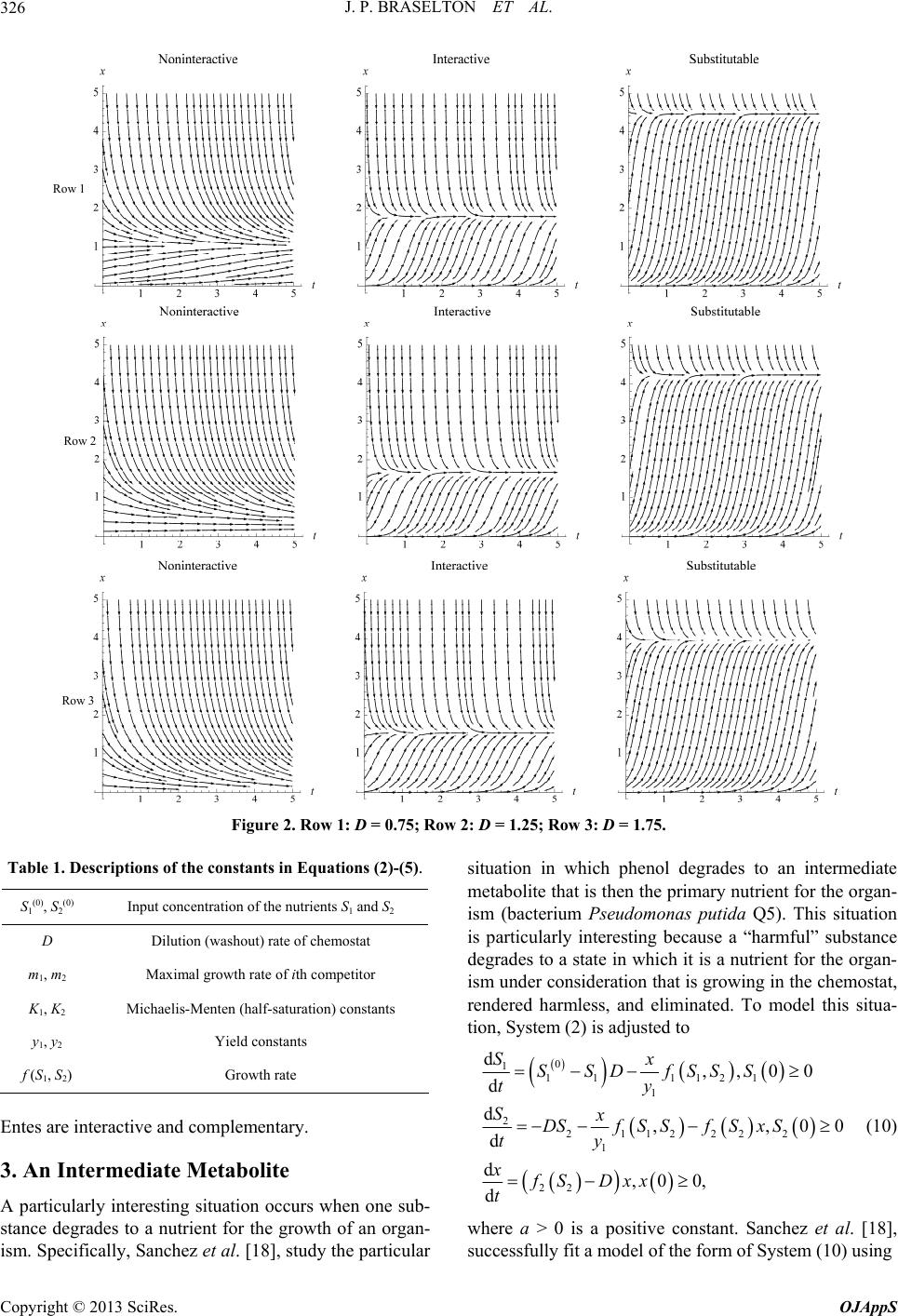

J. P. BRASELTON ET AL. 326
R
ow 1
Row 2
Row 3
Figure 2. Row 1: D = 0.75; Row 2: D = 1.25; Row 3: D = 1.75.
Table 1. Descriptions of the constants in Equations (2)-(5).
S1(0), S2(0) Input concentration of the nutrients S1 and S2
D Dilution (washout) rate of chemostat
m1, m2 Maximal growth rate of ith competitor
K1, K2 Michaelis-Menten (half-saturation) constants
y1, y2 Yield constants
f (S1, S2) Growth rate
Entes are interactive and complementary.
3. An Intermediate Metabolite
A particularly interesting situation occurs when one sub-
stance degrades to a nutrient for the growth of an organ-
ism. Specifically, Sanchez et al. [18], study the particular
situation in which phenol degrades to an intermediate
metabolite that is then the primary nutrient for the organ-
ism (bacterium Pseudomonas putida Q5). This situation
is particularly interesting because a “harmful” substance
degrades to a state in which it is a nutrient for the organ-
ism under consideration that is growing in the chemostat,
rendered harmless, and eliminated. To model this situa-
tion, System (2) is adjusted to





  
0
1
11 1121
1
2
2112222
1
22
d,,00
d
d,,
d
d,0 0,
d
Sx
SSDfSSS
ty
Sx
DSfSSfSx S
ty
xfS Dxx
t
 
00

 
 
(10)
where a > 0 is a positive constant. Sanchez et al. [18],
successfully fit a model of the form of System (10) using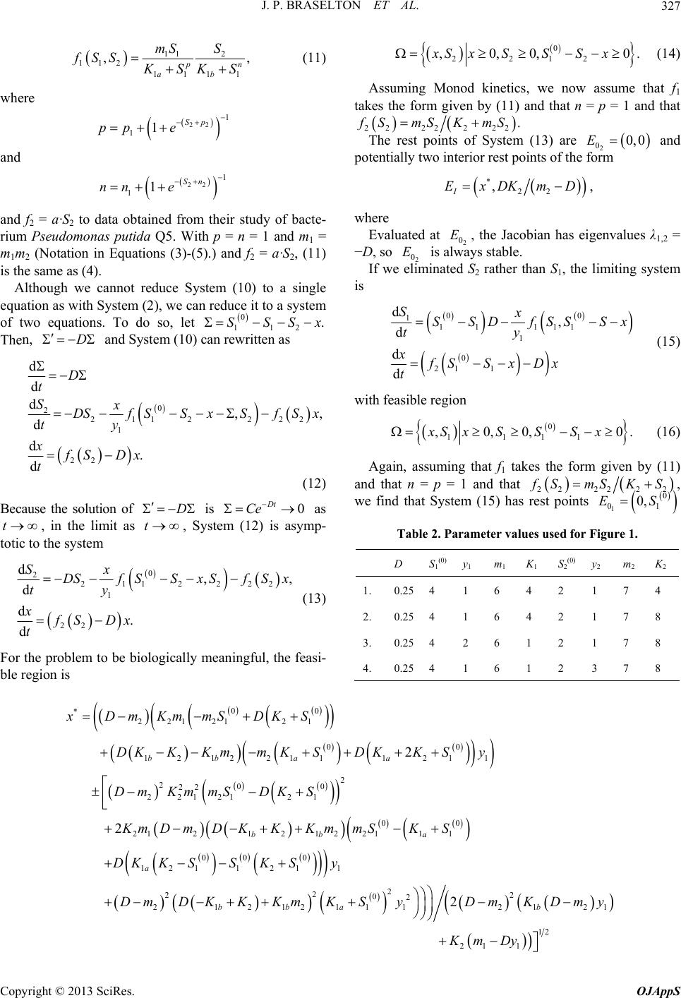

J. P. BRASELTON ET AL. 327

11 2
112
1111
,,
p
n
ab
mS S
fSS
K
SK S

(11)
where


22
1
11Sp
pp e



and


22
1
11Sn
nn e



and f2 = a·S2 to data obtained from their study of bacte-
rium Pseudomonas putida Q5. With p = n = 1 and m1 =
m1m2 (Notation in Equations (3)-(5).) and f2 = a·S2, (11)
is the same as (4).
Although we cannot reduce System (10) to a single
equation as with System (2), we can reduce it to a system
of two equations. To do so, let
Then, and System (10) can rewritten as
 0
112
.SSSx
D

  



 
0
2
2112 222
1
22
d
d
d,,
d
d.
d
D
t
Sx
DSf SSxSfSx
ty
xfS Dx
t

 

(12)
Because the solution of is as
, in the limit as , System (12) is asymp-
totic to the system
D

 
t
0
Dt
Ce  
t



 
0
2
2112222
1
22
d,,
d
d.
d
Sx
DSfSSx SfSx
ty
xfS Dx
t
 

(13)
For the problem to be biologically meaningful, the feasi-
ble region is




0
2212
,0,0,xS xSSSx 0.
(14)
Assuming Monod kinetics, we now assume that f1
takes the form given by (11) and that n = p = 1 and that




2222222
.
f
SmSKmS
The rest points of System (13) are


0, 0E
2
0 and
potentially two interior rest points of the form



*
22
,
I
ExDKmD ,
where
Evaluated at 2
0, the Jacobian has eigenvalues λ1,2 =
−D, so is always stable.
E
2
0
If we eliminated S2 rather than S1, the limiting system
is
E







00
1
11 111
1
0
211
d,
d
d
d
Sx
SSDfSSSx
ty
xfSS xDx
t

 

(15)
with feasible region




0
1111
,0,0,xS xSSSx 0. (16)
Again, assuming that f1 takes the form given by (11)
and that n = p = 1 and that



222222
f
SmSKS,
we find that System (15) has rest points



1
0
01
0,ES
Table 2. Parameter values used for Figure 1.
D S1(0) y1 m1 K1 S2(0) y2 m2 K2
1. 0.254 1 6 4 2 1 7 4
2. 0.254 1 6 4 2 1 7 8
3. 0.254 2 6 1 2 1 7 8
4. 0.254 1 6 1 2 3 7 8

 

 

 








 
 
  
 
 


 









00
*
221 2121
00
1212211121 1
2
200
22
22121 21
00
21212122111
000
121 121 1
2
2
2 2
02
21212111 2
2
2
2
bb aa
bb a
a
bba
xDmKmmSDKS
DKKKmm KSDKKSy
Dm KmmSDK S
KmDmDKKK mmSKS
DKK SSK Sy
Dm DKK Km KSyDm

 


 


 




 


 

 
12
12
21 1
b1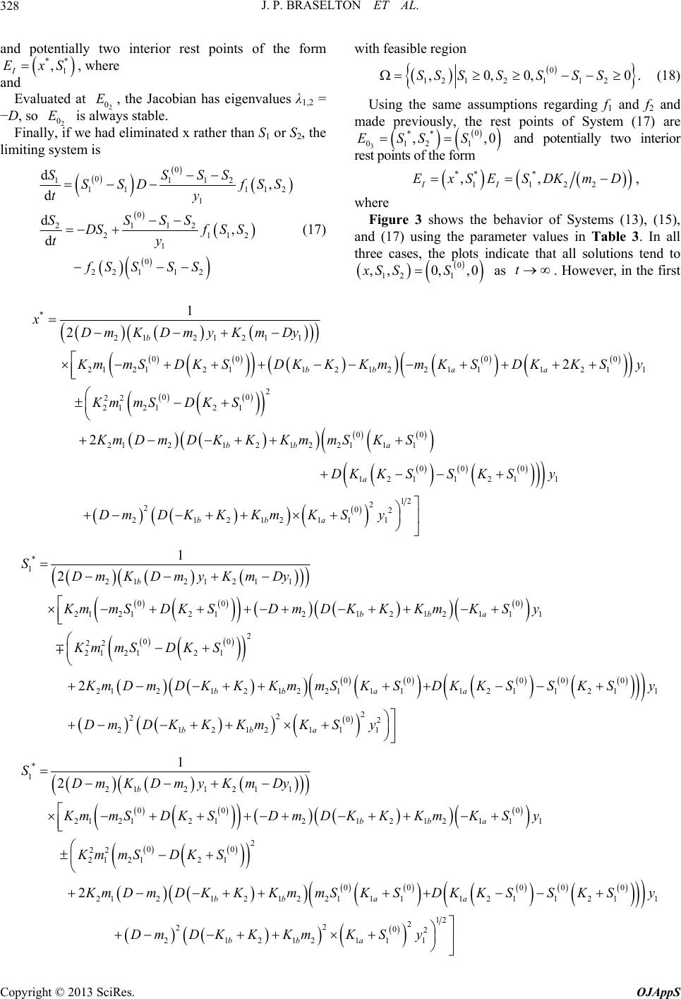
K
Dmy
Km Dy





J. P. BRASELTON ET AL. 328
and potentially two interior rest points of the form
uated at obian has eigenvalues λ1,2 =
1 2

**
1
,
I
ExS, where
and
the JacEval
−D2
0
E,
, so 2
0
E is always stable.
Finally, if we had eliminated x rather than S or S, the
limiting system is










0
112
11 112
1
0
2112
2112
1
0
22 112
,
d
d,
d
S SS
SSDfSS
ty
SSSS
DSfS S
ty
fSSS S



 

(17)
with feasible region
0
1
dS





0
211 2
0,0,0.SSS S  (18)
Using the same assumptions regarding f1 and
m
12 1
,SS S
f2 and
ade previously, the rest points of System (17) are





3
0
**
012 1
,,0ESSS and potentially two interior
rest points of the form




**
1
,
I
ExSE*
122
,
I
SDKmD ,
where re 3 shows the behavior of Systems (13), (15),
an
Figu
d (17) using the parameter values in Table 3. In all
three cases, the plots indicate that all solutions tend to




0
12 1
,,0, ,0xS SS as t. However, in the first
 
 
 
 
 



 
 


  
 
 


 








*
212121 1
00 0
212121121221 1121
2
00
22
21 212 1
00
21212122111
000
121121 1
2
20
2121211
1
2
2
2
b
bb aa
bb a
a
bba
x
DmK Dmy KmDy
0
1
K
m mSDK SDKKKmmKSDKK Sy
Km mSDKS
KmDmDKKK mmSKS
DK KSSKSy
DmD KKKmKS


 






 

 
12
2
1
y



 
 
 


  


 
 
 

 
 


 
 

 



*
1
212121 1
00 0
2121212121 2111
2
00
22
21 2121
00 000
212121 221111211211
2
2
202
21212111
1
2
2
b
bba
bbaa
bba
SDmK DmyKmDy
KmmSD KSDmDKKKmKSy
Km mSDKS
K
mDmDK KKmmSKSDKKSS KSy
DmD KKKmKSy


 





 


 




  

 


 



 


 

 




 

 
 



*
1
212121 1
00 0
2121212121 2111
2
00
22
21 2121
00 000
212121 221111211211
1
2
2
202
21212111
1
2
2
b
bba
bbaa
bba
SDmK DmyKmDy
KmmSD KSDmDKKKmKSy
Km mSDKS
K
mDmDK KKmmSKSDKKSS KSy
DmD KKKmKSy


 






 

 

2



J. P. BRASELTON ET AL. 329
Row 1
Row 2
Row 3
Figure 3. Modeling growth when the nutrient is an intermediate state of the substrate using the parameter values in Table 3.
Table 3. Parameter values used for Figure 3.
D S1(0) y1 m1 K1a K1b m2 K2
1. 0.5 2 1 3 2 2 1 1
2. 0.5 6 1 3 2 2 1 1
3. 0.5 8 1 3 2 2 1 1
two cases there are no interior rest points. While in the
third, when is increased to 8, (3,4), (3,1), and (4,1),
igenvalue of the Jacobian evaluated at the rest point is λ1
= −0.08
More interesting behavior of the systems is illustrated
in Figu 4 where wuseeter values in T le
4he relustrs t when (int con-
tration rate), mr mh ra arin-
c seduilium atescur
aleetuats, te is one ule rest t,
, S1, S2) = (1.76, 7.24, 1), (1.54, 9.46, 1), and (0.260,
4.56, 0.143) as shown in Table 5. However, in the first
two rows of Table 5, (x, S1, S2) = (6.23, 2.76, 1) and
(8.46, 2.54, 1) are stable spirals while in the third row, (x,
S1, S2) = (2.92, 1.93, 0.143) is an unstable spiral.
Thus, depending on the parameter values equilibrium
states may be stable or unstable. Moreover, slight ad-
justments to the parameter values might make a stable
state unstable and vice-versa.
4. Conclusions
In this paper, we have formed a model of gh in a
We have used numerical results to graphically illustrate
le
than do complement-
ta
inte
mentary nutrients. It is possible that if the nutrients are

0
1
S
respectively, are degenerate rest points. For each, one chemostat with two interactive complementary nutrients.
e
33 and the other is λ2 = 0.
re e the paramab
. Tfigu ilatehat

0
1
S
(growt
pu nce
of the subst
, eq
1, o
oc
2
.
tes)e
reaibr st
Inl thr siion hernstabpoin
(x
rowt
differences in the behavior of systems modeling nonin-
teractive compmentary nutrients, interactive comple-
mentary nutrients, and substitutable nutrients. Not sur-
prisingly, we have illustrated that substitutable nutrients
lead to higher population densities
ry nutrients. We have illustrated some surprising dif-
ferences in the behavior of systems modeling noninterac-
tive complementary nutrients and ractive comple-

J. P. BRASELTON ET AL. 330
Row 2
Row 3
Row 1
Figure 4. Modeling growth when the nutrient is an intermediate state of the substrate using the parameter values in Table 4.
Table 4. Parameter values used for Figure 4.
D S1(0) y1 m1 K1a K1b m2 K2
interactive, the organism will attain a stable population
density while if the nutrients are noninteractive, the or-
ganism will become extinct. The simulations indicate
that interactive complementary nutrients frequently lead
to higher population densities than do noninteractive
complementary nutrients. This agrees with the experi-
mental results of Whang et al. [9] that show that com-
plementary substrates (glucose and peptone) significantly
increased hydrogen production by anaerobic hydrogen-
producing bacteria.
A slight adjustment to the system leads to a completely
different interpretation of the model in which the nutrient
the parameter values and slight adjustments to them
can cause a stable state to become unstable and vice
v Thises with experil res-
chez et al. [18], which illustrated that slight ts
of the introrreg
mar et rate
to 1 2) = , 0).
Ma ks tu
carry out many of the calculations as well as generate the
1. 0.5 10 1 3 2 2 1 1
2. 0.5 12 1 3 2 2 1 1
3. 0.25 5 1 8 2 2 2 1
Table 5. Rest points and eigenvalues of Jacobian for Figure
4.
Row x-S1 x-S2 S1-S2 Eigenvalues
of Jacobian
(1.76,7.24) (1.76,1) (7.24,1) −0.359, 0.298
1 ±
0i
.54,9.54,1 − 0
2 8.46,.54,1142
1.26
.26
56
0.29
143 (56,1.43) 0. −0.
(2.92, 0.0401 ±
(6:23, 2:76) (6.24,1) (2.76,1) −0.983
0.85
(1.46) (11) (9.46,) 0.373, .311
2
(8.46,.54) (1) (2) −0. ±
i
(00,
4.)
(6,
0.) 4.230, 224
3
(2.92,1.93) 0.143) (1.93,0.143) 0.919i
is an intermediate byproduct of the substrate. The simu-
lations indicate the equilibrium states are very sensitive
to
ersa. agre thementaults of San
adjustmen
nlet conceation (cspondinto

0
1
S) had
joffects on the
converges
washou
(x, S, S
(when the limit as
(0,

0
St 
e

1
a Thathematic noteboohat the thors used to

J. P. BRASELTON ET AL. 331
figures aby
email request t B
In future studies, wo exam
relationships (competition, pred)
are modeled nces shes
re available from
o Jim
the aut
raselton.
hors sending an
e hope tine how com
ator-prey, and so
petitive
forth
under circumstauch as te.
REFERENCES
[1] S. R. Hansen and S. P. Hubbell, “Single Nutrient Micro-
bial Competition: Agreement between Experimental and
Theoretical Forecast Outcomes,” Science, Vol. 20, No.
4438, 1980, pp. 1491-1493.
http://dx.doi.org/10.1126/science.6767274
[2] H. L. Smith and P. Waltman, “The Theory of the Chemo-
stat: Dynamics of Microbial Competition, Cambridge
Studies in Mathematical Biology,” Cambridge University
Press, Cambridge, 1995.
http://dx.doi.org/10.1017/CBO9780511530043
[3] C. P. L. Grady, Jr., G. T. Daigger and H. C. Lim, “Bio-
logical Wastewater Treatment,” Second Edition, revised
and expanded, Marcel Dekker, New York, 1999.
[4] U. Lendenmann and T. Egli, “Kinetic Models for the
Growth of Escherichia Coli with Mixtures of Sugars Un-
der Carbon-Limited Conditions,” Biotechnology and Bio-
engineering, Vol. 59, No. 1, 1998, pp. 99-107.
http://dx.doi.org/10.1002/(SICI)1097-0290(19980705)59:
1<99::AID-BIT13>3.0.CO;2-Y
[5] G. Stroot, P. E. Saikaly and D. Berther, “Dynamic P.. O
Growth Rates of Microbial Populations in Activated
Sludge Systems,” Journal of Environmental Engineering,
Vol. 131, No. 12, 2005, pp. 1698-1705.
http://dx.doi.org/10.1061/(ASCE)0733-9372(2005)131:12
(1698)
[6]
edings o
of Civil
Engineers, New
[7] J. L. Sherwoo. Skeen and N. B.
19960905)51:
W. Bae and B. E. Rittmann, “Effects of Electron Accep-
tor and Electron Donor on Biodegradation of CC14 by
Biofilms,” Environmental Engineering: Proce
the 1990 Specialty Conference, American Society
f
York, 1990, pp. 390-395.
d, J. N. Petersen, R. S
Valentine, “Effects of Nitrate and Acetate Availability on
Chloroform Production during Carbon Tetrachloride De-
struction,” Biotechnology and Bioengineering, Vol. 51,
No. 5, 1996, pp. 551-557.
http://dx.doi.org/10.1002/(SICI)1097-0290(
5<551::AID-BIT7>3.0.CO;2-B
[8] D. V. Vayenas and S. Pavlou, “Coexistence of Three
Microbial Populations Competing for Three COMPLE-
MENTARY Nutrients in a Chemostat,” Mathematical
Biosciences, Vol. 161, No. 1-2, 1999, pp. 1-13.
http://dx.doi.org/10.1016/S0025-5564(99)00040-1
[9] L.-M. Whang, C.-J. Hsiao and S.-S. Cheng, “A Dual-Sub-
strate Steady-State Model for Biological Hydrogen Pro-
duction in an Anaerobic Hydrogen Fermentation Proc-
ess,” Biotechnology and Bioengineering, Vol. 95, No. 3,
2006, pp. 492-500. http://dx.doi.org/10.1002/bit.21041
[10] P. M. Bapat, S. Bhartiya, K. V. Venkatesh and P. Wangi-
kar, “Structured Kinetic Model to Represent the Utiliza-
tion of Multiple Substrates in Complex Media During
Rifamycin B Fermentation,” Biotechnology and Bioengi-
neering, Vol. 93, No. 4, 2006, pp. 779-790.
http://dx.doi.org/10.1002/bit.20767
[11] P. Champagne, P. J. Van Geel and W. J. Parker, “A Pro-
posed Transient Model for Cometabolism in Ciofilm Sys-
tems,” Biotechnology and Bioengineering, Vol. 60, No. 5,
1998, pp. 541-550.
http://dx.doi.org/10.1002/(SICI)1097-0290(19981205)60:
5<541::AID-BIT4>3.0.CO;2-Q
[12] W. Bae and B. E. Rittmann, “A Structured Model of
Dual-Limitation Kinetics,” Biotechnology and Bioengi-
neering, Vol. 49, No. 6, 1996, pp. 683-689.
http://dx.doi.org/10.1002/(SICI)1097-0290(19960320)49:
6<683::AID-BIT10>3.3.CO;2-E
[13] M. M. Ballyk and G. S. K. Wolkowicz, “Exploitive Com-
petition in the Chemostat for Two Perfectly Substitutable
Resources,” Mathematical Biosciences, Vol. 118, No. 2,
1993, pp. 127-180.
http://dx.doi.org/10.1016/0025-5564(93)90050-K
[14] G. J. Butler and G. S. K. Wolkowicz, “Exploitive Com-
petition in a Chemostat for Two Complementary, and
Possible Inhibitory, Resources,” Mathematical Biosci-
ences, Vol. 83, No. 1, 1987, pp. 1-48.
http://dx.doi.org/10.1016/0025-5564(87)90002-2
[15] S-B. Hsu, K-S. Cheng and S. P. Hubbell, “Exploitive
Competition for Two Complementary Nutrients in Con-
tinuous Cultures,” SIAM Journal on Applied Mathematics,
Vol. 41, No. 3, 1981, pp. 422-444.
http://dx.doi.org/10.1137/0141036
[16] S.-B. Hsu and Y.-H. Tzeng, “Plasmid-Bearing, Plas-
mid-Free Organisms Competing for Two Complementary
Nutrients in a Chemostat,” Mathematical Biosciences,
Vol. 179, No. 2, 2002, pp. 183-206.
http://dx.doi.org/10.1016/S0025-5564(02)00105-0
[17] H. R. Thieme, “Convergence Results and a Poincaré-
Bendixson Trichotomy for Asymptotically Autonomous
Differential Equations,” Journal of Mathematical Biology,
Vol. 30, No. 7, 1992, pp. 755-763.
http://dx.doi.org/10.1007/BF00173267
[18] J. L. Garcia-Sanchez, B. Kamp, K. A. Onysko, H. Bud-
man and C. W. Robinson, “Double Inhibition Model for
Degradation of Phenol by Pseudomonas Putida Q5,” Bio-
technology and Bioengineering, Vol. 60, No. 5, 1998, pp.
560-567.
http://dx.doi.org/10.1002/(SICI)1097-0290(19981205)60:
5<560::AID-BIT6>3.0.CO;2-L
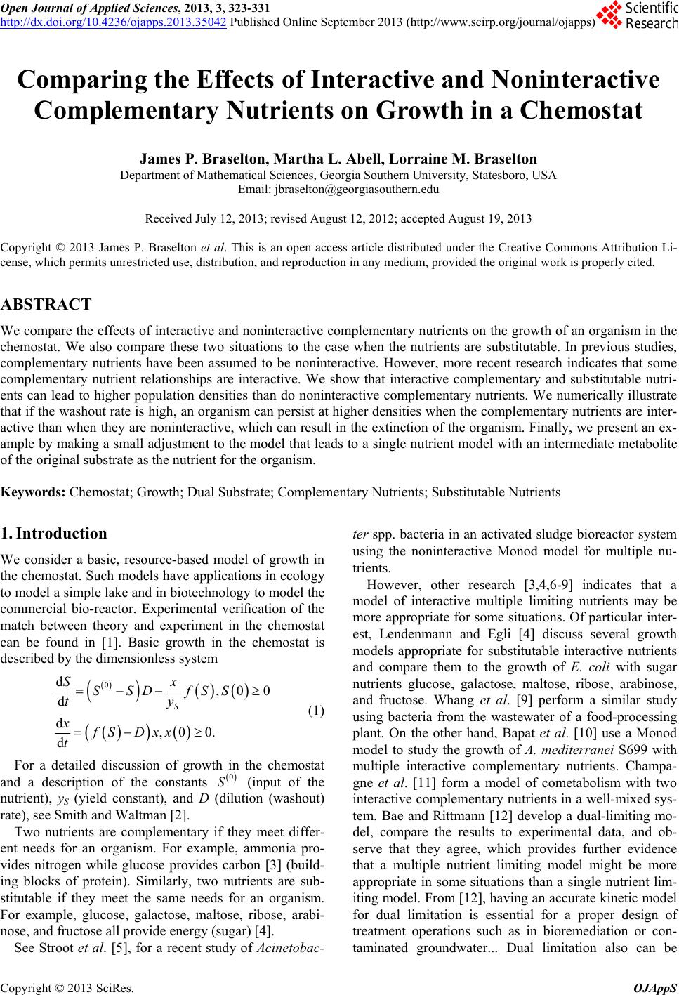