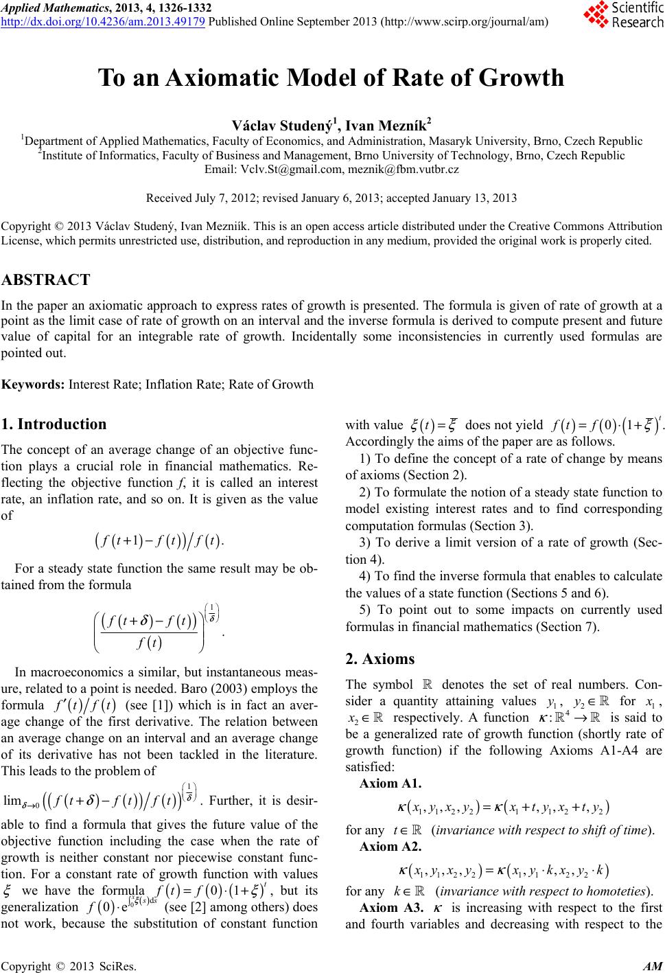Applied Mathematics, 2013, 4, 1326-1332
http://dx.doi.org/10.4236/am.2013.49179 Published Online September 2013 (http://www.scirp.org/journal/am)
To an Axiomatic Model of Rate of Growth
Václav Studený1, Ivan Mezník2
1Department of Applied Mathematics, Faculty of Economics, and Administration, Masaryk University, Brno, Czech Republic
2Institute of Informatics, Faculty of Business and Management, Brno University of Technology, Brno, Czech Republic
Received July 7, 2012; revised January 6, 2013; accepted January 13, 2013
Copyright © 2013 Václav Studený, Ivan Mezniík. This is an open access article distributed under the Creative Commons Attribution
License, which permits unrestricted use, distribution, and reproduction in any medium, provided the original work is properly cited.
ABSTRACT
In the paper an axiomatic approach to express rates of growth is presented. The formula is given of rate of growth at a
point as the limit case of rate of growth on an interval and the inverse formula is derived to compute present and future
value of capital for an integrable rate of growth. Incidentally some inconsistencies in currently used formulas are
pointed out.
Keywords: Interest Rate; Inflation Rate; Rate of Growth
1. Introduction
The concept of an average change of an objective func-
tion plays a crucial role in financial mathematics. Re-
flecting the objective function f, it is called an interest
rate, an inflation rate, and so on. It is given as the value
of
()() () ()
1.
f
tftf+− t
For a steady state function the same result may be ob-
tained from the formula
()() ()
()
1
.
ft ft
ft
δ
δ




+−



In macroeconomics a similar, but instantaneous meas-
ure, related to a point is needed. Baro (2003) employs the
formula
() ()
f
tft
′ (see [1]) which is in fact an aver-
age change of the first derivative. The relation between
an average change on an interval and an average change
of its derivative has not been tackled in the literature.
This leads to the problem of
()() () ()
()
1
0
lim ftft ft
δ
δ
δ



→+− . Further, it is desir-
able to find a formula that gives the future value of the
objective function including the case when the rate of
growth is neither constant nor piecewise constant func-
tion. For a constant rate of growth function with values
ξ
we have the formula
()( )()
01 t ft f
ξ
=⋅+
d, but its
generalization
()
()
0
0e
x
s
s
f
ξ

⋅ (see [2] among others) does
not work, because the substitution of constant function
with value
()
t
ξξ
= does not yield
()( ) ()
01 t ft f
ξ
=⋅+ .
Accordingly the aims of the paper are as follows.
1) To define the concept of a rate of change by means
of axioms (Section 2).
2) To formulate the notion of a steady state function to
model existing interest rates and to find corresponding
computation formulas (Section 3).
3) To derive a limit version of a rate of growth (Sec-
tion 4).
4) To find the inverse formula that enables to calculate
the values of a state function (Sections 5 and 6).
5) To point out to some impacts on currently used
formulas in financial mathematics (Section 7).
2. Axioms
The symbol denotes the set of real numbers. Con-
sider a quantity attaining values , for 1

1
y2 y∈
x
,
2 respectively. A function is said to
be a generalized rate of growth function (shortly rate of
growth function) if the following Axioms A1-A4 are
satisfied:
x∈4→: κ
Axiom A1.
()(
112 21122
,,,,, ,
)
x
yx yxtyxty κκ =++
for any (invariance with respect to shift of time). t∈
Axiom A2.
()(
112 2112 2
,,,, ,,
)
x
yx yxykxyk κκ =⋅⋅
for any ( invariance with respect to homoteties). k∈
Axiom A3.
κ
is increasing with respect to the first
and fourth variables and decreasing with respect to the
C
opyright © 2013 SciRes. AM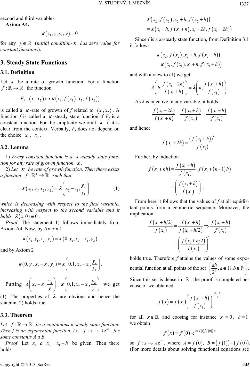

V. STUDENÝ, I. MEZNÍK 1327
second and third variables.
Axiom A4.
()
12
,, ,0xyx y κ =
for any ( initial condition-y∈
κ
has zero value for
constant functions).
3. Steady State Functions
3.1. Definition
Let
κ
be a rate of growth function. For a function
the function
:f→
()() ( ()
121122
:,, ,,
f
)
F
xxxfxxfx κ 
is called a -rate of growth of f related to
κ
12
,
x
x. A
function f is called a -steady state function if Ff is a
constant function. For the simplicity we omit if it is
clear from the context. Verbally, Ff does not depend on
the choice
κ
κ
1
x
, 2
x
.
3.2. Lemma
1) Every constant function is a -steady state func-
tion for any rate of growth function .
κ
κ
2) Let be rate of growth function. Then there exists
a function such that
κ
f2 :→
()
2
112 221
1
,,, ,
y
xyx yxx y κλ

=−



)
(1)
which is decreasing with respect to the first variable,
increasing with respect to the second variable and it
holds .
()
,0 0x λ ≡
Proof: The statement 1) follows immediately from
Axiom A4. Now, by Axiom 1
()(
112 21212
,,,0,, ,
x
yx yyxxy κκ =−
and by Axiom 2
()
2
12 122 1
1
0,,,0,1,, y yxxyxx y κκ

−= −


.
Putting 22
21 21
11
,0,1,,
yy
xx xx
yy
λκ

−= −





we get
(1). The properties of
λ
are obvious and hence the
statemnt 2) holds true.
3.3. Theorem
Let be a continuous κ-steady state function.
Then f is an exponential function, i.e.
:f→
:e
B
x
fx A for
some constants A a B.
Proof: Let 1
x
a 21
x
xh=+ be given. Then there
holds
)
()( ) ()
() ( ()
222 2
111 1
,,,
,,2,2
xfxx hfx h
x
hf xhxhf xh
κ
κ
++
=++ ++
Since f is a κ-steady state function, from Definition 3.1
it follows
()( ) ()
()( ) ()
222 2
111 1
,,,
,,,
x
fx x hfx h
x
fx x hfx h
κ
κ
++
=+ +
and with a view to (1) we get
()
()
()
()
1
21
11
,, .
f
xh

+fxh
hh
fx h fx
λλ

+
=


+

As λ is injective in any variable, it holds
()
()
()
()
()
()
121
2
12
1
f
xhfxhfx+++
==
h
fx hfxfx+
and hence
()
()
()
()
2
1
1
1
2.
fx h
fx hfx
+
+=
Further, by induction
()
()
() ()
()
()
()
1
11
1
1
1
1
.
n
fx h
f
xnh+= fx nh
fx
fx h
fx
+⋅ +−

+
=


From here it follows that the values of f at all equidis-
tant points form a geometric sequence. Moreover, the
implication
()
()
()
()
()
()
()
()
111
11 1
2
1
1
2
2
2
f
xhfxhfxh
fxfx hfx
fx h
fx
+++
=
+

+
=


holds true. Therefore f attains the values of some expo-
nential function at all points of the set ,,
2b
ah ab

∈∈



.
- Since this set is dense in , the proof is completed be
cause of we obtained

() () ( )()
1
1
1
1
x
x
h
fx h
fx fx
−
−

+
=fx




for all and coosing for instance
we obt
x∈
ain 10x=, 1h=
() ()
()() ()
ln 10
0e
f
fx
fx f⋅ =⋅
so :e
B
x
f
xA, where
()
0
A
f=,
t solving fun
()
()
()
()
10Bf f=−.
ctional equations see (For more details abou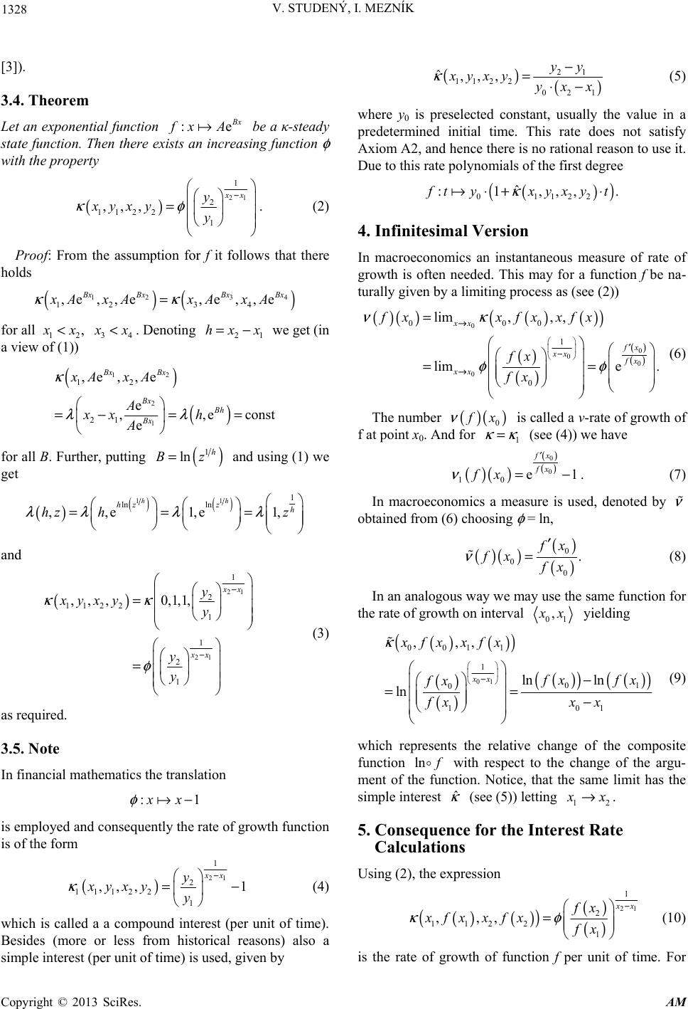

V. STUDENÝ, I. MEZNÍK
1328
[3]).
. Theorem 3.4
Let an exponential function :e
B
x
fx A be a κ-steady
state function. Then there exing function φ sts an increasi
with the property
()
21
1
2
1122
1
,,, y xyx yy κφ


=

 
. (2)
xx−



Proof: From the assumption for f it follows that there
holds
4
() ()
3
12
123 4
,e ,,e,e , ,e
Bx Bx BxBx
xA xAxAxA κκ =
for all 12
x
x<, 34
x
x<. Denoting 21 hx x=− we get (in
a view of (1))
()
()
12
2
2
Bx
Bh
x λ

=−

1
12
1
,e , ,e
e
,,econst
e
Bx Bx
Bx
xAxA
A
x h
A
κ
λ = =


for all B. Further, putting
()
1
ln h Bz= and usin1) we
get
g (
()
() ()
11
1
ln ln
,,e1,e1,
hh
hzz h
hz hz λλλλ


===

 

 

and
 

()
21
21
1
2
112 2
1
1
2
1
, ,,0,1,1,xx
xx
y
xyx yy
y
y
κκ
φ
−
−



=

 




=

 

(3)
as required.
3.5. Note
athematics the translation In financial m
:1
x
x
φ
−
is employed and consequently the rate of growth function
is of the form
()
21
1
2
11122
1
,,, 1xyx yy κ =−

 (4)
which is called
xx
y−

a a compound interest (per unit of time).
Besides (more or less from historical reasons) also a
simple interest (per unit of time) is used, given by
)
()
(
21
112 2
021
ˆ,,, yy xyxyyxx κ
−
=⋅− (5)
where y0 is preselected constant, usually the value in a
predetermined initial time. This rate does not satisfy
Axiom A2, and hence there is no rational reason to use it.
Due to this rate polynomials of the first degree
( ()
01122
ˆ :1,,,
)
.
f
ty xyxy κ ⋅+ ⋅t
4. Infinitesimal Version
In macroeconomics an instantaneous measure of rate of
growth is often needed. This may for a function f be na-
turally given by a limiting process as (see (2))
()( )( )() ()
()
()
()
()
0
0
00
00
lime .
xx fx
φφ
→
==


000
1
lim,,,
xx
fx
xx fx
fxxfx xfx νκ
→
 ′

−

=




fx




(6)





The number
() ()
0
f
x ν
is called a ν-rate of growth of
f at point x0. An(see (4)) we have d for κκ =1
()
()
()
()
0
0
10
e1
fx
fx
fx ν
′
=−.
In macroeconomics a measure is used, denoted by
(7)
ν

obtained from (6) choosing φ = ln,
(
()
)
() ()
0.
0
0
f
x
fx
f
x (8)
In an analogous way we may use the
th
ν
′
=

same function for
e rate of growth on interval 01 ,
x
x yielding
() ()
()
()
()
()
()
()
()
0011
,,,xfxxfx
01
1
01
0ln
ln xx
10
1
ln
f
x
fx


−




==



which represents the relative change of the composite
function
fx− (9)
fx x x−



κ

ln
f

he fun
terest
with respect to the change of the argu-
ment of tction. Notice, that the same limit has the
simple in (see (5)) letting
ˆ
κ
12
x
x→.
5. Consequence for the Interest Rate
Calculations
thUsing (2),e expression
) () () (()
()
21
1
1122
,,, 2
1
x
x
f
xfxxfx
κφ
−

=

x
fx (10)
time. For

is the rate of growth of function f per unit of

V. STUDENÝ, I. MEZNÍK 1329
ins ents how the state a dead account
drawals) depends on time as-
1f time and the unit of time is
a year, then
tance, if f repres
(neither deposits nor with
suming x, x are moments o
2
() () ()
1122
,,,
x
fxx fx κ
ereas if we choose in (2)
is the interest rate
per a year, wh
()
1,
t
xx φ =−
we get (denoting the resulting function by t
κ )
() ()
()
() ()
21
1
2
1
1
, 1
xx
t
fx
xf x
κ
−

−


which is a compound interest related t
1 2 2
,,
xx fxf =



o time segment
. Besides, it holds
21
tx x=−
11
11.
t
κκ

=+−
t


 (11)
It is known, that banks at the beginning of t past
century (due to practical reasons stemming from the
he
nonexistence of computers) used to find the value 1t κ
for small 1t the approximation by Taylor polynomial
of the first degree of function (11) which gives the result
()
()
1.2
1
11
11
tO
t
κ
κκ



+−=+
interval of adding of interests” was introduced with the
clause, that if the current interval was shorter than that
(where O is Bachmann-Landau big-O). Consequently,
supposing interest rate was known for some time interval
(e.g. a month), the interest rate for shorter intervals (e.g.
a day) was calculated dividing by 30 instead of as the
30th root. To legalize this inaccuracy, the notion of “an
under assumption, the interest will be calculated multi-
plying only by a linear part of the increment of the inter-
est rate. Hence function f representing the state of ac-
count being in a steady state was changed from exponen-
tial to piecewise linear having with the original exponen-
tial curve common only breaking points. This practice is
still surviving, despite banks use software that is defi-
nitely capable to calculate the roots. The reason rests
(probably) with the shortage of management theoretical
competence. The difference between the exact value and
its approximation, i.e. an error of approximation is an
increasing function when time approaches to infinity
having finite limit e1
κ
κ −− because it holds
lim11lim11
e1.
t
t
tt
tt
κ
κ
κ
κκ
→∞ →∞

 

+−=+−
 

 

=−
(12)
This limit is employed in a number of books on finan-
cial mathematics, its interpretation although is rather
problematic. When we calculate compound interest and
manipulate with a compound interest as with a simple
interest in such a way that we divide time interval in
equidistant subintervals and apply the interest tha
linear part of the approximation for these subintervals,
we obtain the result, whose limit for the number of sub-
in
t is the
tervals approaching to infinity is given by formula (12)
A magic appearance of Euler constant in this calculation
gave birth the notion of continuous compounding. It may
be simply verified that it is in fact a compound interest,
where in formula (4) the value
()
1
ln 1 κ + instead of 1 κ
is applied. The number
()
1
ln 1 κ + may be obtained as a
rate of growth when putting φ = ln in (2) and then by
limiting we get
ν
 as in (8).
6. Inverse Problem
Let us use for the rate of growth formula (7) and denote
1
ν
ν = with argument t in the sequel. Then we have for a
fixed t0
()
()
()
()
0
0
0e1
ft
ft ν =−. (13)
ft
′
Supposing f is given, then (13) is the formule to find
rnatively, when ν is given, then
)
t
or
the rate of growth ν. Alte
(13) is a differential equation to get the function f. This
equation can be rearranged equivalently to
()
()
()(
ln1 lntf ν
′
+= 
() () () ()
ln 1
f
ttft ν
′=+⋅
with the solution
()
() ()
()
()
0ln1 d
e0,
tss
ft f
ν +

= (14)
where
()
s
ν
nt s.
is the interest rate per unie
me Performing the same calculation for
t of time at th
mo
ν
 (see
, we get
0
(8))
() () ()()
00
f
tftft ν
′
=

with the solution
()
()
()
0d
e
tss
ft f
ν

= 0.
h
el
instance if we substitute a constant interest
rate in (15), we do not obtain the formor a com-
pound interest! The following example illustrates the use
Example. We assume that the inflation rate per a unit
of time (e.g. a year) at time 0 and time
po
(15)
Althougthe formula (15) is clearly simplier than (14),
it has disadvantage, because it yields quantitativy bad
results. For
ula f
of formula (14).
1 is known. Sup-
se that the inflation rate per unit of time at time 0 is 0.1
and 0.2 at time 1. Deliberate on the inflation rate on in-
terval 1,0 . It is evident that this depends on the

V. STUDENÝ, I. MEZNÍK
1330
changes of the inflation rate on 1,0 . Consider the fol-
lowing four cases of the inflation rate:
()
1
0.1, if1u
ι
<

0.2, if1,u≥

u=
()
2
20.1,
10
u
u ι =+
()
30.1,
10
u
u ι =+
()
0.1, if0u
u
ι
≤

=
40.2, if0.u>

Notice that the first and the last cases are trivial—the
rate is constant and the interval has a unit length and thus
the inflation rate should be the same constant. The gen-
eral formula must give the same result. By (14) we have
()( )
() () ()
()
1
0ln1d
10eiuu ff
ι
1.

=⋅ − (16)
Applying (16) we get consecutively (setting )
+
()
01f=
()
()
()
()
() ()
()
()
()
12
0
1
0
ln 1.110 d
ln 1.110 d
for2 :1e10.132945354
for3: 1 e10.149637533
uu
uu
if
if
+
+


== −=
== −=


()
()
()
1
0
1
0
ln 1.1 d
ln 1.2 d
for1:1e1 0.1
for4 :1e10.2.
u
u
if
if


== −=
== −=
Now, applying (15) we obtain results
1
0
12
0
1
0
1
0
0.1d
1100.1d
1100.1d
0.2d
e1 0.105170918
e1 0.142630812
e1 0.161834243
e1 0.221402758.
u
uu
uu
u
+
+




−=
−=
−=
−=
The results are surprisingly not equal (particularly the
fir ent failure. For-
mula for the future value of the compound interest in
case of constant interest rate is given by
.
st and the last one) which is an evid
()( )()
01 t ft f
ξ
=⋅+ (17)
In case of piecewise constant interest rate, i.e. if
i
I
me are the values of constant interest rate per year on ti
intervals
(
1
,
ii
tt
+, 0,,in=, then the interest rate per
(
1
0,
n
ii
itt
+
=
 is given by
()
()
6.1. Theorem
Fo n
4) for aiecewise c
Proof: Ass
1
1
0
1.
ii
ntt
i
i
I+
−−
=
+
∏ (18)
rmula (17) is a special case of formula (18) for a co-
stant interest rate and formula (18) is a special case of
formula (1 ponstant interest rate.
ume
()
tI
ν
= is constant. Then there holds
()
()
() ()
(
(
0ln1
ln 1dln 1
eee
tI
Iu tI
)
)
()
1
tt
I
+ +⋅+
===+
and hence the fi
let
rst part of the statement holds true. Now
ν
be piecewii
I
se constant possessing values on
intervals
(
1
,
ii
tt
+, 0, ,in= and A
χ
be a character-
istic function of set A. We have
()
()
1
,
ii i
tt
tI ιχ
+
=⋅
 and
hence
(
( (
, 0ln 1
e
t
tt
ii
χ
+
+⋅

)
) )
() () () ()(
1
1
1
01
d
ln 1ln 11ln1
00
ee
i
n
ii
ii
iii i
Iu
tItI ntt I
ii
−
+
=+

+− +−


−⋅+

==

==
∏
)
()
()
6.2. Theorem
Formula (14) is a limit case of formula (17).
Proof: First we show, that for every continuous func-
tion f defined on a closed interval, there exists a sequence
of piecewise constant functions
()
11
0
11
ln 1
e1
tt
ii ii
i
i
nn
tt
I
i
I
−
++
=
−−
−
+
== +
∏∏
and the proof is completed.
i
ξ
with the property
i
f
ξ
→. Let f be a continuous funtion. Due to the as-c
sumption
()
Dom
f
is the c
tive real number. For eve
ompact set. Let be posi-
ry

()
mDo
x
f
at
()
()
∈ we find a
such thneighborhood O
()
x
()
()
2
f
Ox ⊂Of x
.
()
{
}
()
Dom
x
f
Ox ∈ forms a covering of
(
Dom
)
f
. Choose
a finite subcovery Ω and define
() ()
min Diam
UU
δ
∈Ω
=,
where
()
Diam U is a diameter of U. Consider a parti-
tion of
()
Dom
f
given by n disjoint subintervals
i
()
n
i
J
 of the length
δ . In every subinterval i
J
 we
choose a pd denote
()
ii
oint xi, an
y
fx=. Furer, define
()
i
th
x
y ζ =
 for all i
x
J∈. Then
()
Dom for every
x
f∈
it holds
() )(
fx x≤ and fo ζ −
r 1
2n
n
ξζ
= the above
sfied. Since the functionproperty is satial
() (
0ln 1d
:e
t
)
s
s ι
ι
+

Φ
is continue topology of uniform convergence,
t
()
()
()
lim lim
ii
ψψ
→∞ →∞
Φ=Φ =ΦΨ
ous in th
we ge
roof is completed
unding
As an impact of the preceding considerations let us point
to the issue of simple compouding. Simple compounding
ii
and the p.
7. Interest Rate of Simple Compo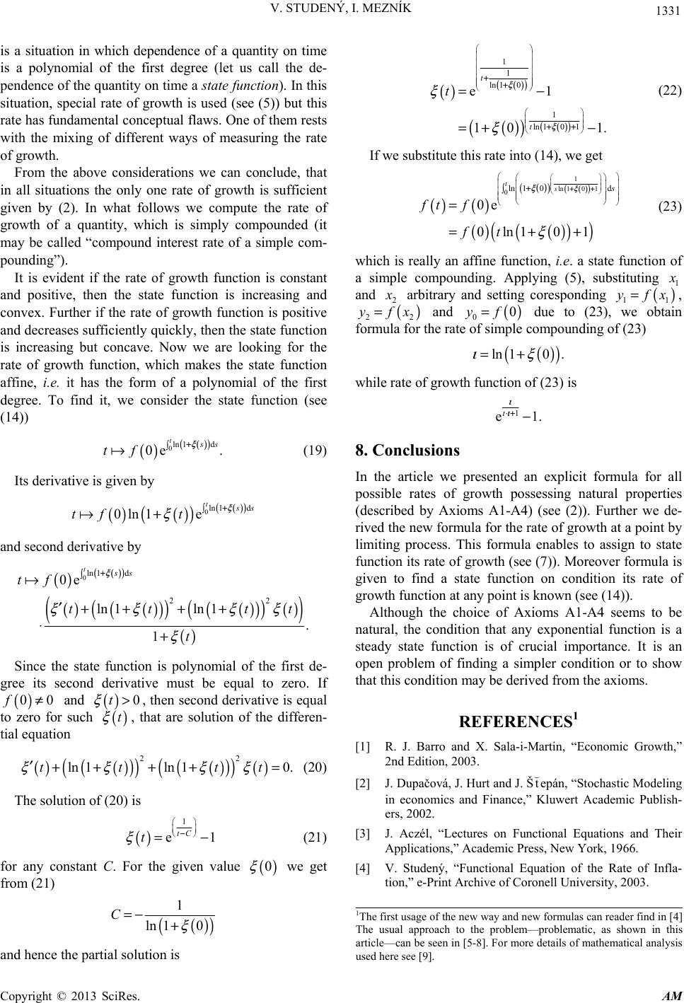

V. STUDENÝ, I. MEZNÍK 1331
is a situation in which dependence of a quantity on time
is a polynomial of the first degree (let us call the de-
pendence of the quantity on time a state funcon). In this
situation, special rate of growth is used (see )) but this
tual flaws. One of them rests
with the mixing of different ways of measuring the rate
ti
(5
rate has fundamental concep
of growth.
From the above considerations we can conclude, that
in all situations the only one rate of growth is sufficient
given by (2). In what follows we compute the rate of
growth of a quantity, which is simply compounded (it
may be called “compound interest rate of a simple com-
pounding”).
It is evident if the rate of growth function is constant
and positive, then the state function is increasing and
convex. Further if the rate of growth function is positive
and decreases sufficiently quickly, then the state function
is increasing but concave. Now we are looking for the
rate of growth function, which makes the state function
affine, i.e. it has the form of a polynomial of the first
degree. To find it, we consider the state function (see
(14))
()
() ()
0ln1d
0e .
t
s
s
tf
ξ +

 (19)
Its derivative is given by
() () ()
() ()
0ln 1d
0ln1 e
t
s
s
tf t
ξ
ξ
+

+
and second derivative by
()
()
()
() ()
()
()
()
()
()
()
()
()
0ln 1d
0e
tss
tf
ξ +


22
ln 1ln 1
1
tt
t
ξξ
ξ
′++ ++
⋅+
Since the state function is polynomial of the first de-
gree its second derivative must be equal to zero. If
and , then second derivative is equal
at are solution of the differen-
(
The solution of (20) is
.
tt
ξξ
()
00f≠
tial equation
()
0t ξ >
to zero for such
()
t ξ , th
() () ()
()
() ()
()
()
22
ln 1ln 10.tt tt ξξ ξξ
′++ ++=
20)
()
1
e1
tC
t ξ

−

=− (21)
onstant the given value
()
0 ξ we get
from (21)

for any c C. For
()
()
1
ln 10
C
ξ
=− +
()
()
()
()
()
()
()
1
1
ln 10
1
ln 101
10 1
t ξ
ξ



++
=+ −
e1
.
t
t
ξ
ξ




+


+


=−
If we substitute this rate into (14), we get


(22)
()( )
()
() () ()
() ()
()
()
1
ln 101
0ln 10d
0e
0ln10 1
ts
s
ft f

ft
ξ
ξ
ξ



++





+



 

=+ +
(23)
which is really an affine function, i.e. a stat
a simple compounding. Applying (5), substituting


 
=
e function of
1
x
and 2
x
arbitrary and setting coresponding
()
11
y
fx=,
()
22
y
fx=
fo
and due to (23),
while rate of growth function of (23) is
()
00yf= we
(23)
obtain
rmula for the rate of simple compounding of
() ()
ln 10. ιξ =+
1
e1
t
ι
ι ⋅+ − .
e a
e de-
rived the new formula for the rate ofrowth at a point by
limiting process. This formula enables to assign to state
reover formula is
given to find a state function on condition its rate of
growth function at any point is kwn (see (14)).
Although the choice of Axioms A1-A4 seems to be
n that any exponential function is a
tion,” e-Print Archive of Coronell University, 2003.
8. Conclusions
In thrticle we presented an explicit formula for all
possible rates of growth possessing natural properties
(described by Axioms A1-A4) (see (2)). Further w
g
function its rate of growth (see (7)). Mo
no
natural, the conditio
steady state function is of crucial importance. It is an
open problem of finding a simpler condition or to show
that this condition may be derived from the axioms.
REFERENCES1
[1] R. J. Barro and X. Sala-i-Martin, “Economic Growth,”
2nd Edition, 2003.
[2]  J. Dupačová, J. Hurt and J. Štepán, “Stochastic Modeling
in economics and Finance,” Kluwert Academic Publish-
ers, 2002.
[3] J. Aczél, “Lectures on Functional Equations and Their
Applications,” Academic Press, New York, 1966.
[4] V. Studený, “Functional Equation of the Rate of Infla-
1The first usage of the new way and new formulas can reader find in [4]
The usual approach to the problem—problematic, as shown in this
article—can be seen in [5-8]. For more details of mathematical analysis
used here see [9].
and hence the partial solution is

V. STUDENÝ, I. MEZNÍK
1332
http://arxiv.or
Z, Praha, 2000.
cs, Vol. 10-III,” Academic Press, New
lassification Codes:
SC (Mathematics Subject Classification)
g/abs/math/0307395
[5] J. C. Van Horne, “Financial Markets, Rates and Flows,”
Prentice Hall, Englewood Clifs, 1978.
[6] R. C. Merton, “Continuous Time Finance,” Blackwell,
Cambridge, 1992.
[7] I. Karatzas and S. Shreve, “Methods of Mathematical
Finance,” Springer, New York, 1998.
[8] T. Cipra, “Mathematics of Securities,” H
[9] J. Dieudonné, “Treatise on Analysis, Vol. III, Pure and
Applied Mathemati
York, London, 1972.
C
M
26A12, Rate of growth of functions, orders of infinity, slowly varying functions
62P20, Applications to economics
39B22, Equations for real functions
91B02, Fundamental topics (basic mathematics, methodology; applicable to economics in general)
91B28, Finance, portfolios, investment
91B24, Price theory and market structure
ctions 34A05, Explicit solutions and redu
JEL (Journal of Economic Literature)
E4, Money and Interest Rates: General (includes measurement and data)
Structure of Interest Rates
C43, Index Numbers and Aggregation
E43, Determination of Interest Rates; Term
C02, Mathematical Methods
C63, Computational Techniques
C65, Miscellaneous Mathematical Tools