Journal of Geographic Information System, 2011, 3, 18-49
doi:10.436/jgis.2011.31003 Published Online January 2011 (http://www.SciRP.org/journal/jgis)
Adjusting Second Moment Bias in Eigenspace Using
Bayesian Empirical Estimators, Dirichlet Tessellations
and Worldview I Data for Predicting Culex
Quinquefasciatus Habitats in Trinidad
Models for West Nile Vectors
Benjamin G. Jacob1, Dave D. Chadee2, Robert J. Novak1
1School of Medicine, Division of Infectious Diseases, University of Alabama at Birmingham,
Birmingham, Alabama, USA
2Department of Life Sciences, University of the West Indies, St. Augustine, Trinidad and Tobago, West Indies
Received October 24, 2010; revised November 12, 2010; accepted December 23, 2010
Abstract
Temporally weighted regression models with a spatial autoregressive component may estimate nonlinearities
in spatiotemporal-sampled data of Culex quinquefasciatus, a major vector of West Nile Virus (WNV) which
can help implement control strategies by determining optimal predictors associated to prolific habitats. The
design of this kind of mixed model can specifically incorporate spatial autocorrelation whilst including the
influence of other aspatial predictor variables. Currently, the lack of an estimation theory that allows for het-
eroscedasticity and corresponding joint hypothesis testing in the presence of spatial dependence in georefer-
enced Cx. quinquefasciatus habitat data is a serious shortcoming in WNV research. In this paper we used
spatially lagged and simultaneous autoregressive models based on multiple predictor variables of immature
Cx. quinquefasciatus and Worldview 1 (WV-1) data to help implant a remote habitat-based surveillance sys-
tem in Trinidad. Initially, we used Geomatica Ortho Engine® v. 10.2 for extracting a Digital Elevation Model
(DEM) from the WV-1 raw imagery. Results of the DEM analyses indicated a statistically significant inverse
linear relationship between total sampled Cx. quinquefasciatus data and elevation (m) (R2 = −0.439; p <
0.0001), with a standard deviation of 10.41. Additional field-sampled information was derived using data
from an orthogonal grid-matrix constructed in an ArcInfo 9.3® and overlaid onto the WV-1 data. A unique
identifier was placed in the centroid of each grid cell. Univariate statistics and Poisson regression models
were then generated using the georeferenced covariates in SAS/GIS®. Coefficient estimates were also used to
define expectations for prior distributions in a Bayesian estimation matrix using Markov Chain Monte Carlo
(MCMC) specifications. A spatial residual trend analyses was then performed using autocorrelation indices
which linked tabular data in SAS PROCLMIXED® with the egg-raft count data in ArcInfo®. The estimation
matrix identified prolific habitats based on the covariate distance to the nearest house. An Ordinary
kriged-based interpolator was then constructed in Geostatistical Analyst Extension of ArcGIS 9.3® based on
the adjusted Bayesian estimates. For total Cx. quinquefasciatus egg-raft count, first order trend was fitted to
the semivariogram at a partial sill of 5.931 km, nugget of 6.374 km, lag size of 7.184 km, and a range of
31.02 km using 12 lags. We assessed the performance accuracy of the interpolation procedures based on the
magnitude and distribution of errors between observed and model-predicted values using Voroni tessella-
tions. These residuals divided the space between the individual georeferenced Cx. quinquefasciatus habitats
by XY coordinates in 2-dimenisional space which revealed that the geophysical parameter error residuals in
the interpolation model were within normal statistical limitations. Newer GIS software and WV-1 data can
generate highly accurate predictive Cx. quinquefasciatus habitat distribution models which can target prolific
habitats of based on field-sampled count data. Our results suggest it may be unnecessary to manage all Cx.

B. G. JACOB ET AL.
19
quinquefasciatus habitats to obtain significant reductions in incidence and prevalence of WNV in Trinidad.
Keywords: Culex Quinquefasciatus, Trinidad, West Nile Virus, Worldview 1, ArcGIS®
1. Introduction
West Nile virus (WNV) is among the Culex-borne en-
cephalitides in the Flavivirus genus. The virus cycles
between birds and mosquitoes, while horses, humans,
and a number of other vertebrates are considered inci-
dental hosts. Since WNV first appeared in the Western
Hemisphere in New York in 1999, it has spread rapidly
across the North American continent, causing large
numbers of human cases with neurologic disease and
death and even greater amounts of milder disease char-
acterized principally by fever and rash [1]. West Nile
Virus has been spreading southward into the Caribbean
Basin and Latin America as well, where its public health
impact remains poorly understood [2]. The virus was
first detected in 2001, in Jamaica and the Cayman Is-
lands. Thereafter, serological evidence of WNV trans-
mission has been accumulating. Cross-reactive WNV
antibodies in humans have been detected from Mexico,
the Bahamas, and Cuba, in horses from Guadalupe,
Mexico, Central America, Puerto Rico, Colombia, and
also in resident birds from the Dominican Republic and
Venezuela. In November 2006, 4 serologically confirmed
human WNV encephalitis cases were reported in Argen-
tina. West Nile Virus may be following the same patterns
of southward dissemination as other arboviruses into the
Caribbean and Central and South America via migratory
birds.
There have been attempts to develop and implement
WNV surveillance in the Caribbean but, unfortunately
present systems in the region are unprepared to track
WNV spread. For example, in Guadeloupe, extensive
surveillance for WNV infection demonstrated a high
seroprevalance in equines in 2003, despite no human or
equine case being reported. A protocol for epidemiol-
ogical surveillance for WNV has been developed through
a collaborative electronic working tool posted on the
Caribbean Animal Health Network (CaribVET) website
(www.caribvet.net). CaribVET is a collaboration of vet-
erinary services, diagnostic laboratories, research insti-
tutes, universities, and regional/international organiza-
tion to improve animal health in the Caribbean through
exchange of information and data management. Improv-
ing collaborations and information dissemination for
understanding WNV epidemiology is vital; however,
WNV surveillance and diagnostics in the Caribbean re-
quires tools for regional data analyses. Unfortunately, to
date there have been virtually no significant findings in
any established WNV surveillance programs in tropical
America. In september 2007, WNV infection detected by
polymerase chain reaction (PCR) in post-mortem brain
tissue taken from an encephalitic horse and by virus iso-
lation from a dead bird confirmed WNV transmission in
southwest Puerto Rico but, since then there have been no
isolates reported from other areas in Central and South
America or the Caribbean.
The explanation for the paucity in WNV detection in
tropical America may be the lack of active WNV sur-
veillance. One would hypothesize that the likelihood of
identifying WNV cases would be maximized in the Car-
ibbean Basin, given its location in the flight paths of in-
fected migratory birds. However, due to cross-immunity
of WNV with other tropically endemic Flaviruses such
as St. Louis encephalitis, it is possible that WNV has not
been able to establish persistent enzootic foci in the re-
gion, so that reported serological evidence may be caused
by frequent but unsuccessful virus reintroductions. Re-
gardless, presently a WNV mosquito habitat-based in-
tervention surveillance system using a vigorous quantita-
tive assessment of field and remote-sampled data is war-
ranted for countries of the Caribbean.
A main challenge in devising an effective West Nile
surveillance program in regions of the Caribbean; how-
ever, is the lack of sufficient empirical knowledge on the
spatiotemporal patterns of Culex quinquefasciatus larval
habitats and their underlying contribution to the adult
population. The main tropical vector for WNV in birds
and people is Cx. quinquefasciatus in the Southeastern
United States and the Caribbean [3]. Previous research
has revealed that Cx. quinquefasciatus abundance will
vary significantly in different areas due to hydrologic
regime and the proximity to habitats and blood-meal
hosts [4-7]. These factors are not evenly distributed spa-
tiotemporally, so it is logical to expect a variation in ab-
undance and distribution of virus-positive mosquitoes
within different ecosystems in the Caribbean.
Recently, the use of remote sensing (RS) and GIS for
the quantitative prediction of geographical distributions
of agent, reservoir, and vector species has been advo-
cated to augment traditional WNV mapping methods
[4,5,8]. For example, the United States Geological Sur-
vey (USGS) and Center of Disease Control (CDC) have
employed GIS and RS to prepare interpretive maps
showing WNV activity in many regions of North America
(http://www.cdc.gov/ncidod/dvbid/westnile/resources/wn
vguidelines1999.pdf). Common GIS/RS technology for
WNV data analyses include: 1) time series overlay
analyses of thematic data and spatial intersection, 2)

B. G. JACOB ET AL.
20
buffer generation and neighborhood analysis, 3) vec-
tor-based grid generation and network analysis; and, 4)
surface modeling [9]. Once an area has been imaged,
associations between risk variables and environmental-
sampled covariates can be quantified using the spatial
data analysis capabilities of GIS for implementing a
WNV mosquito surveillance system [9-11].
Quantification of vector-host interactions incorporated
on Land Use Land Cover (LULC) maps generated in GIS
time series overlay analyses suggest that Culex habitat
productivity vary greatly over short distances, depending
on the space and time at which field measurements are
made [5,12-15]. For example, Jacob et al. (2009a) gener-
ated a land use land cover (LULC) classification in Erdas
Imagine based on Landsat-7 ETM+ data acquired July
2003 and Landsat-5 TM data acquired July 1991 for
examining two ornithophillic mosquito vector species
Culex pipiens and Culex restuans in residential areas of
Urbana-Champaign, Illinois [4]. A maximum likelihood
unsupervised classification and LULC detection was
performed using a cross-tabulation detection method and
a grid-based algorithm stratified by drainage for detection
of environmental predictors associated to field-sampled
egg-raft abundance count data. The resulting LULC
change matrix revealed that between 1991 and 2003
there was a total of 12.1% LULC change in the study site.
Of 20,166 egg-rafts sampled, 76.7% was in land cover
classified as maintained urban followed by 14.8% in
maintained non-urban. The well-drained stratum har-
bored 56.4% of the total sampled data. Additionally, a
remote stratification of the urban land cover site based on
QuickBird visible and near infrared (NIR) data revealed
that 83.3% of the egg-raft distribution was in LULC
classified as residential high canopy coverage. In another
study, Jacob et al. (2009b) constructed multiple geospa-
tial models based on LULC and meteorological variables
to predict adult abundance of the same Culex species in
Des Planes mosquito abatement district in northern Cook
County, Illinois [5]. An ecological database of the study
site was constructed in ArcGIS 9.2® also using multitem-
poral QuickBird visible and NIR data overlaid with total
adult Culex abundance and WNV infection rates from 15
georeferenced gravid traps sampled weekly from May
2002 to October 2005. A regression analyses of LULC
parameters revealed that adult Culex abundance in the
georeferenced gravid traps was positively associated with
temperature and negatively associated with precipitation.
In 2002, the overall accuracy of the model was 73.3%,
65.1% in 2003, 47.2% in 2004 and 60.0% in 2005.
Temperature and precipitation explained > 80.1% of the
variation in each of the models. Estimates from the mul-
tivariate analysis also revealed that land cover that was
classified as forest LULC along with middle range built
environment (< 40.1%) predicted heightened infected
vector activity. Because abiotic factors such as LULC are
measurable in GIS using submeter resolution data, these
pre-epidemic abiotic signatures may be quantified for
predicting arboviral epidemic transmission in isolated
areas of the Caribbean. These epidemic signatures may
be tracked, measured, quantified, and presented visually
to help forecast human arboviral epidemics. While re-
mote models of the observed spread of WNV have been
used to evaluate potential vector and host mechanisms of
dispersal and to define the suitability of the various
landscape features and meteorological variables for
mosquito transmission of WNV in many portions of the
US, there is no literature using LULC and high resolu-
tion satellite data for evaluating ecologically sampled Cx.
quinquefasciatus habitats in any region of the Caribbean.
Recently, digital elevation models (DEMs) have
become popular with the use of GIS for surface modeling
flood and swamp water mosquito abundance in many
different geographic regions [16-18]. A digital elevation
model (DEM) is a digital file consisting of terrain
elevations for ground positions at regularly spaced
horizontal intervals. It is a digital representation of
ground surface topography which is usually represented
as a raster or as a triangular irregular network. DEMs
include a number of production strategies for determining
terrain-related parameters associated to prolific Cx.
quinquefasciatus habitats such as manual profiling from
photogrammetric stereo models, digitizing of contours,
digitizing topographic map contour plates, converting
hypsographic and hydrographic tagged vector files and
also for performing autocorrelation via automated
photogrammetric systems. To obtain DEMs from satellite
images for determining vector amplification and host
population dynamics for mapping the spatiotemporal
distribution of WNV from high resolution data two
methods are possible: along-track stereoscopy from the
same orbit using fore and aft images and across-track
stereoscopy from two adjacent orbits [16]. The four
possibilities of stereo image processing for DEM
generation are Fore-Aft, Fore-Nadir, Aft-Nadir and
Fore-Aft-Nadir images as a pair [19]. The simultaneous
acquisition of along-track stereo data has a strong
advantage in terms of radiometric variation versus the
multi-date acquisition of across-track stereo data which
has been traditionally employed in past research for
identifying terrain-related explanatory covariates of
floodwater mosquito habitats [20]. The across-track
approach has been applied frequently since 1980, first
with Landsat from two adjacent orbits, then with SPOT
using across-track steering capabilities and finally with
IRS-I C/D. But these satellite data were limited due to
spatial resolution. Fortunately, along-track stereoscopy

B. G. JACOB ET AL.
21
has recently gained renewed popularity using higher
resolution satellite data systems including JERS-i’s
optical sensor(OPS), German Modular Opto-electronic,
Multi-Spectral Stereo-Scanner (MOMS), ASTER, IKON-
OS, QuickBird, Orthoview, SPOT-5, FORMOSAT II,
Cantosat and the latest addition of Digitalglobe’s
Worldview (WV)-1. These data can define georeferenced
terrain covariates associated with prolific Cx. quinque-
fasciatus habitats. For example, Jacob et al. (2010) used
multispectral QuickBird data and DEM-based GIS
methods to evaluate stream flow direction for determining
satellite-derived characteristics of drainage basin physio-
graphic predictors associated with Culex erraticus, a
mosquito vector of eastern equine encephalitis virus
(EEEV) and Northern Cardinals, an avian host associated
with WNV and EEEV in Tuskegee, Alabama [16].
Eastern equine encephalitis virus is a virulent arbovirus
maintained in an enzootic cycle between local avian
fauna and ornithophilic mosquitoes in coastal regions of
the eastern United States [1,14,16]. Euclidian distance-
to-nearest hydrological body was calculated as the
distance in geo-space from a grid cell to a stream grid
cell defined by a Stream Raster Grid. A Terrain Analysis
using a DEM (i.e., TauDEM) was then performed in
ArcGIS 9.2® to retrieve multiple geomorphological
parameters. Additionally, a three-dimensional model of
the study area was constructed based on the DEM using
ArcScene extension of ArcGIS®. A Pearson correlation
analyses computed the ratio of covariance between the
sampled variables to the product of their standard
deviations. Substituting estimates of the covariances and
variances based on the Cx. erraticus samples provided
the sample correlation coefficient which revealed
significant inverse linear relationships between the total
field-sampled adult count data and elevation (R2 =
−.4711; p < .0001) with a standard deviation (SD) of
11.16. The analyses of the Northern Cardinal data and
elevation also revealed a similar statistical relationship
(R2 = −.5831; p < .0001) with a SD of 11.42. Even
though the usefulness of selected static catchment
predictor covariates (e.g., stream, density, and slope) in
assessing Culex habitats has been verified in previous
research, characteristics of drainage networks and basin
physiographic parameters have not been applied in
modeling WNV mosquito abundance and distribution in
any country of the Caribbean.
Predictive interpolation algorithms have also not been
used for forecasting productive Cx. quinquefasciatus
habitats based on field and remote-sampled data in any
country of the Caribbean. One of the most powerful and
potentially valuable GIS/RS vector mosquito data mod-
elling mechanisms is that of automated prediction. Gen-
erally, given relevant spatiotemporal field and re-
mote-sampled explanatory predictor variables with ap-
propriate annotation, a WNV mosquito model can be
constructed for making accurate forecasts of one or more
dependent “target” quantities of interest. These quanti-
ties of interest may be continuous real values (a scenario
often referred to as regression” or “interpolation”), in
vector mosquito data analyses or, it can be in the format
of discrete labels (“aquatic habitat classification” or
“habitat distribution pattern recognition”). Both these
cases are referred to as “supervised learning” in the
GIS/RS vector mosquito data learning vernacular. Pre-
dictive interpolation algorithms can also map urban
variation in vectors based on differentials in environ-
mental-sampled parameters which can identify and vali-
date models linking human ecological factors, while
controlling for potential spatial autocorrelation in model
residuals [21-25]. Spatial autocorrelation, the correlation
among values of a single variable strictly attributable to
their relatively close positions on a two-dimensional sur-
face is frequently encountered in the analyses of spatio-
temporal georeferenced vector mosquito data [4,8,21,
26,27]. Autocorrelation violates the ordinary least
squares (OLS) assumption that the error terms are un-
correlated. While it does not bias the OLS coefficient
estimates in a predictive vector mosquito habitat distri-
bution model, the standard errors tend to be underesti-
mated and the t-scores overestimated when the autocor-
relations of the errors at low lags are positive [16].
Kriged-based interpolation may analyze spatiotempo-
ral-sampled WNV mosquito data in the presence of
fine-scale autocorrelation. Kriging is mathematically
related to regression analyses. Both theories derive a best
linear unbiased estimator based on assumptions of co-
variance and make use of the Gaussian-Markov theorem
to prove independence amongst georeferenced vector
mosquito data exploratory parameters [26]. Kriging vec-
tor mosquito data is commonly made by interpolation of
a single realization of a randomized study area based on
field and remote observations in multivariate environ-
mental-sampled datasets. Under the regionalized as-
sumption, local habitat variation is not generally un-
structured but, it is spatially dependent at some scale as
georeferenced points within a given habitat distance
apart depend on one another in a statistical sense (16)
Any variable is stationary when its distribution is invari-
ant under translation, that is, the stationary region is the
location to make estimates (26). Stationary variables
provide a preliminary model decision for uncertainty
about the sample value at a specific sampled habitat lo-
cation z(x) (16). For any space lag (h) increment in a
particular direction, the distribution of z(x1), z(x2) ... z(xn)
habitat based observations is the same as that of z(x1 + h),
z(x2 + h)...z(xn + h), where z(x) is regarded as the sum of

B. G. JACOB ET AL.
22
three terms: (1) mean, drift or trend, (2) random depend-
ent variable plus (3) error (16) This, however, requires
the first two moments (i.e., mean and variance) to be
constant. This spatial homogeneous region in the distri-
bution of the georferenced Cx. quinquefasciatus habitats
then will make random functions homogeneous and
self-repeating in space. The variance of the random spa-
tial variable will equal covariance at zero lag habitat dis-
tance (σ2 = C (0), while the covariance between z(x) and
z(x + h) becomes σx,x+h = σ2f(h) = C (h) (16). This means
that the stationary covariance only depends on the sam-
pled habitat distance and direction between two sampled
habitats and not on their georeferenced locations, or the
second order stationary assumption. Hence, the expected
difference between sampled values at two georferenced
Cx. quinquefasciatus habitat locations separated by dis-
tance h is zero. If E (μ(x)) = m then z(x) = m + e(x) and
E (z(x) - z(x + h)) = 0 (23). Covariance at h lag habitat
distance then will be E{(z(x) - m)(z(x + h)-m)} = E(z(x)
x z(x + h)) - m2 = Cov(h), being that z(x) the value at x
sampled habitat site, z(x + h) the value at x sampled
habitat site plus h lag habitat distance is based on m rep-
resenting the overall mean and E() symbolizing the ex-
pected value (16). Although the covariance does not exist
theoretically in a predictive vector mosquito habitat dis-
tribution model, the variance of the difference between
two sampled habitat locations will be assumed to be pre-
sent, as it does not depend on the georeferenced location
and Var (z(x + h) - z(x)) = E({z(x + h) - z(x)} = 2γ(h),
being E(z(x) - z(x + h) = 0. That is, differences between
sampled habitat sites are merely a displacement function
between them (i.e, the intrinsic hypothesis). The γ(h) (i.e.,
dissimilarity average function) will be the key tool for
the structural interpretation of the predicted Cx. Quin-
quefasciatsus habitats as well as for uncertainty estima-
tion parameters. Mathematically, the variogram is de-
fined as γ(h) = 0.5xVar(z(x + h) - z(x) (26). Since, the
mean of z(x + h) - z(x) is zero for intrinsic variables then
the variance is just the mean square difference. Conse-
quently, the variogram for a predictive vector habitat
distribution model is as follows: γ(h) = 0.5xE{(z(x + h) -
z(x))2}(16). These predictive interpolation vector mos-
quito habitat distribution models can measure unknown
local mean habitat values as having a local linear or
quadratic trend by combining regression of the depend-
ent variable (e.g., larval/pupal count data) based on aux-
iliary variables, such as terrain-related parameters (i.e.,
slope), RS imagery, and thematic maps, with kriged re-
siduals where auxiliary predictors are used directly to
solve the weights. For instance, in our previous example
of research conducted in Tuskegee, Alabama for exam-
ining vector-host activities of Culex erraticus, a kriged-
based interpolator was also constructed in Geo-statistical
Analyst Extension of ArcGIS 9.2® for predicting prolific
habitats based on adult abundance count data [16]. For
total adult Cx. erraticus count, a first-order trend ordi-
nary kriging process was fitted to the semivariogram at a
partial sill of 5.764 km, nugget of 6.114 km, lag size of
7.472 km, with a range of 32.62 km using 12 lags, sug-
gesting that this species forage several kilometers beyond
their habitats. The values that the semivariogram model
attains at the range (i.e., the value on the y-axis) is called
the sill, while the nugget or nugget variance, C0, occurs
when a curve is fitted to the set of points that lie within
the range and sill and the model used has a non-zero in-
tercept [28].
Furthermore, to improve interpolation accuracy in a
kriged-based algorithm, predictive mean standard error
distributions can be quantified for attaining asymptoti-
cally optimal predictors. Traditional kriging is motivated
by an expected squared prediction error from a stochastic
model [28]. Presently many algorthmitic paradigms of
computational geometry have been applied efficiently in
Geomatics and GIS using Dirichlet/Voronoi/Thiessen
tessellation techniques for assessing interpolation models
for quantifying the maximum error variance and the ex-
tended prediction variance [28]. A Voronoi diagram is a
special kind of decomposition of a metric space deter-
mined by distances to a specified discrete set of objects
in the space, (e.g., dataset of Culex habitat ground refer-
ence coordinates). Generalization towards dynamic op-
erations and kinematic motion have been investigated for
about a decade using Dirichlet neighborhood analyses.
Voroni residuals are amenable to assessment of good-
ness-of-fit tests in a predictive vector mosquito habitat
distribution models as they are approximately Gamma
distributed and tend to be far less skewed than Pearson’s
residuals and other residual diagnostic tests [16]. Such
tessellations have been used in grid generation in vol-
umes and surfaces, data compression, image segmenta-
tion and edge detection, optimal allocation of resources,
optimal quadrature rules, optimal representation, quanti-
zation, finite difference tests and finite volume schemes.
Unfortunately, there is no published literature using in-
terpolation algorithms or Dirichlet tessellations for quan-
tifying spatial error and predicting habitat locations using
georeferenced spatiotemporal-sampled predictor vari-
ables in WNV mosquito research for any country of the
Caribbean.
In this research, we generated multiple predictive
geospatial models using field and remote-sampled ex-
planatory variables of Cx. quinquefasciatus habitats in
Trinidad. Elucidation of variability in mosquito produc-
tivity requires spatial accounts of oviposition processes
[29]. Indeed, this is important because of the recent iden-
tification of sero-positive horses and domestic birds in

B. G. JACOB ET AL.
23
Trinidad [2]. Presently there is no remote habitat-based
intervention for early detection of WNV activity in any
regions of the Caribbean or Central and South America.
A remote habitat-based intervention may provide early
detection of arboviral activity by providing useful infor-
mation for projection of the potential course of WNV
transmission and also other arthropod-born viral diseases
(e.g., St Louis encephalitis, Venezuelan equine encepha-
litis) later in the season while unraveling the environ-
mental factors associated with the maintenance and es-
tablishment of enzootic cycles in Trinidad and in other
countries of the neotropics.
For mosquito larval control to be effective, however, it
may be crucial to quantify individual sampled habitat
variation to maximize control efforts. For example, the
importance of variation in mosquito production among
breeding sites in design of control programs is now
broadly accepted in suppressing domestic container-
breeding Aedes aegypti, a mosquito vector of Dengue in
Trinidad. This research involved quantifying population
densities of A. aegypti in four towns using standard
house-to-house inspections of all water-holding contain-
ers to determine whether persistently positive containers
and premises existed over a three-month period in the
wet season, from May to July 2002. From a total of
1,503 houses inspected, 15% were positive with 3% per-
sistently positive over the three month period and classi-
fied as ‘key premises’. From a total of 24,439 containers
inspected, 1.3% were positive for A. aegypti larvae and
pupae. Of 17 container types inspected, only water
drums (54%), buckets (22%), tubs and basins (8%), wa-
ter tanks (5%), brick holes (4%), and tires (2%) were
significant larval habitats (P < 0.001) producers. The role
that key premises play in the introduction and reinfesta-
tion of A. aegypti-free communities was determined. The
results suggested that A. aegypti control programs could
be more cost effective and sustainable by targeting ef-
forts on key premises and key containers to control
mosquito densities and dengue transmission while re-
ducing manpower needs and insecticide use.
In this research, we constructed an autocovariate error
matrix in SAS/GIS® for spatially targeting estimates
generated from individual sampled Cx. quinquefasciatus
habitat data. In our Bayesian model we did not assume
that the georeferenced predictor variables were condi-
tionally independent, as is commonly the case in hierar-
chical generalized linear model (HGLM) construction
practices for predicting WNV mosquito habitats. In our
Bayesian network we assumed that the variables were
conditionally independent. In practice, this assumption
may not hold for WNV mosquito habitat models and
may give rise to incorrect inferences. Violation of the
assumption of statistical independence will give rise to
incorrect model specifications [28]. Thus, we proposed
the creation of a hidden node for modeling the depend-
ency in the spatiotemporal-sampled parameters. In order
to determine the conditional probability matrices for the
hidden node, we used a gradient descent method. The
objective function to be minimized was the squared-error
between the measured and computed values of the in-
stantiated nodes. Both forward and backward propaga-
tion were used to compute the node probabilities for
quantifying the dependence in the data. We also re-
stricted our attention to the simultaneous autoregressive
Gaussian spatial process and the autoregressive Gaussian
response model (i.e., the spatial lag model), for quanti-
fying latent autocorrelation error components in the
Bayesian uncertainty estimates. We assumed that ob-
served parameter error estimation patterns in the re-
sponse variable decomposed into three statistically inde-
pendent components: 1) a systematic spatial trend com-
ponent that could be specified by a parsimonious set of
exogenous variables; 2) a stochastic signal that reflects
either an underlying spatial process and/or a set of miss-
ing exogenous factors with an inherent spatial pattern;
and, 3) independent white-noise disturbances. A specific
subset of eigenvectors was then used to determine local
and regional variation in the field and remote-sampled
covariates by capturing dependencies among distur-
bances generated from the Bayesian probabilistic model.
Eigenvectors are a special set of vectors associated with
a linear system of equations (i.e., a matrix equation)
[4,5,8,10].
We constructed our remote habitat-based intervention
by adoption of a landscape approach to elucidate mecha-
nisms underlying Cx. quinquefasciatus productivity. Our
landscape perspective was based on multiple georefer-
enced explanatory variables of individual sampled habi-
tats to determine their role in WNV disease transmission
in Trinidad. Arguably, our framework evolved from the
traditional concept of regression models generated from
LULC covariates for identification of hot zones (i.e.,
cluster), but our remote habitat-based intervention also
focused on critical spatial autoregressive modifications
of the georeferenced predictors. We developed our mod-
els to emphasize the role of oviposition foraging in Cx.
quinquefasciatus in Trinidad. Habitat-based interventions
should emphasize the link between foraging behaviors of
egg-laying mosquitoes and the availability of breeding
sites in evaluation of environmental management pro-
grams [29]. The basic assumption in our models was that
heterogeneity in immature productivity was substantially
large among Cx. quinuefaciatus habitats and that the
number of productive habitats was relatively fewer than
that of unproductive ones in focal areas. Untargeted in-
terventions are inefficient because habitats are randomly

B. G. JACOB ET AL.
24
selected without consideration of the distribution of pro-
duction (29). Spatially targeting prolific breeding habitats
using a remote habitat-based intervention may reduce Cx.
quinuefaciatus populations in Trinidad and help imple-
ment a cost-effective surveillance mechanism. Therefore,
our objectives of this research were to: 1) construct a
DEM to identify terrain-related explanatory covariates
associated with spatiotemporal-sampled mosquito data; 2)
generate regression models to determine statistical sig-
nificance associated with the sampled covariates, 3)
quantify latent autocorrelation components in model re-
sidual variance estimates generated from an eigenfunc-
tion decomposition spatial filter algorithm; and, 4) de-
velop spatial interpolation models of potential prolific
habitats site based on field-sampled count data. Although
the discussion is centered on WNV vectors specifically in
Trinidad, the framework and derived guidelines in this
research may be applicable to integrated control pro-
grams for other mosquito species and insect-borne dis-
eases in other regions.
2. Material and Methods
2.1. Study Site
The island of Trinidad is the most southerly part of the
Lesser Antilles located at approximately 10° north lati-
tude and 15 km from the eastern coast of Venezuela. The
geology, flora and fauna are typical of the adjacent South
American mainland [31,32]. Trinidad is approximately
80 km from north to south and is on average 60 km wide,
roughly rectangular in shape with large promontories on
the northwest and southwest of the country. The climate
of Trinidad is tropical with a “rainy” season between
May and November and a “dry” season from December
to May. Details about climate, physical features, vegeta-
tion, and population size have been previously described
[33,34].
2.2. Mosquito Egg Sampling
The Cx. quinquefasciatus habitat population was sur-
veyed by counting the number of egg-rafts deposited in
oviposition traps. Field sampling was conducted from
July 2008 to July 2009. One hundred and fifty two tem-
porary, permanent, and semi-permanent mosquito larval
habitats in the study site were mapped and classified, and
recalibrated using a CSI-Wireless differential corrected
global positioning systems (DGPS) Max receiver which
yields a positional error of .179 m (+/− 392 m) [35]. Wa-
ter bodies were inspected for Cx. quinquefasciatus egg-
rafts. Oviposition traps were located in shady areas
around residences and municipal buildings, as well as the
edge of parks and woodlots.
2.3. Habitat Base Mapping
Initially, Landsat images were collected using SLC-off
mode (http://edc.usgs.gov/#Find_Data/Products_and_
Data_Available/ETM). We used the USGS Global
Visualization Viewer (GloVis) system (http://glovis.usgs.
gov/) to search for images for performing a land cover
classification. Path 233/row 53 covered the Trinidad
study area. Unfortunately, the images acquired from
GloVis, were all cloudy, due to the climate conditions of
the island. Cloudy image is an issue for remote
classification and change detection for identification of
mosquito habitats [24]. We did find three Landsat 7
passes of path 233/row 53 which were less than 10%
cloud free. Theses collection periods were April 30, May
16, and June 1, 2005. These data; however, were not able
to discriminate the land cover due to poor resolution (i.e.,
30m resolution) associated with the overlaid geo-
referenced Cx. quinquefasciatus habitats coordinates.
We acquired WV-1 data (www.digitalglobe .com) for
the study site on July 2010. Operating at an altitude of
496 kilometers, WV-1 has an average revisit time of 1.7
days and is capable of collecting up to 750,000 km2 per
day of half-meter resolution imagery. The satellite is
equipped with state-of-the-art geolocation accuracy
capabilities and exhibits stunning agility with rapid
targeting and efficient in-track stereo collection. Various
collection sizes of surveying are available: frame mode,
route survey (along coastline, roads and linear objects),
areal survey (60 × 60 km), and stereoscopic areas on a
single pass as well (www. digitalglobe.com).
In this research, the WV-1 imagery was radiometrically
and sensor corrected but was not projected to a plane using
a map projection or datum. The sensor correction blended
the pixels from all the detectors into synthetic arrays to
form the image of the study site. The geolocation accu-
racy specification of the data was 4.0 to 5.5 m CE 90 at
nadir excluding terrain and off-nadir effects. The im-
agery was delivered at full-swath cut into 14 km lengths.
The WV-1 imagery was classified using the Iterative
Self-Organizing Data Analysis Technique (ISODATA)
unsupervised routine in ERDAS Imagine v.8.7™ (At-
lanta, USA) which is commonly used to classify land
covers associated with disease foci [18,26,29]. The im-
ages were co-registered manually using ground control
points (GCPs) and by applying a first order polynomial
algorithm with a nearest neighbor re-sampling method.
The Universal Transverse Mercator (UTM) Zone 20P
datum WGS-84 projection was used for all of the spatial
datasets.
Base maps were prepared from the field-sampled Cx.

B. G. JACOB ET AL.
25
quinquefasciatus habitat data and WV-1 imagery for the
study site using the DGPS ground coordinates. We gen-
erated GIS data layers in the vector shapefile format,
ArcInfo® Coverage format and raster GRID format for
use in the GIS software package ArcGIS v 9.3®. We
constructed a discrete tessellation of the region using a
digitized grid-based algorithm (Figure 1). For remote
identification of vector mosquito habitats the first step is
often to construct a discrete tessellation of the region
[36]. A unique identifier was placed in each grid cell.
Each Cx. quinquefasciatus habitat/polygon was assigned
a unique identifier. Field attribute tables were then asso-
ciated to the polygons.
2.4. Environmental Data Analyses
Base maps were also generated using the spatiotemporal-
sampled Cx. quinquefasciatus habitat data which was
stored in a Vector Control Management System® (VCMS)
(Clarke Mosquito Control Products, Inc. 159 N. Garden
Avenue, Roselle, IL 60172) database. The VCMS sup-
ported the mobile field data acquisition in the study site
through a PocketPC™. All two-way, remote synchroni-
zation of data, geocoding and spatial display were proc-
essed using the embedded GIS Interface Kit™ that was
built using ESRI’s MapObjects™ 2 technology. The
VCMS database plotted and updated the DGPS ground
coordinates of the Cx. quinquefasciatus habitats and
supported exporting data in spatial format in which any
combination of the sampled habitats and explanatory
covariates were described in ESRI shapefile format for
use in GIS. The database displayed this information onto
a user-defined field base map.
2.4.1. Spatial Hydrological Model
The latest version of PCI Geomatics Orthoengine® soft-
ware was used to generate a DEM using the WV-1 data
and the georeferenced Cx. quinquefasciatus habitat co-
variates (Figure 2). OrthoEngine offers an industry-
leading variety of control sources including, manual en-
try, geocoded imagery, geocoded vectors, chip database,
digitizing tablet, or a text file (www. pcigeomatics.com).
We used the DGPS coordinates to orient the images to
our map coordinate system. We used PCI Geomatics
OrthoEngine to extract the DEM. PCI software sup-
ports automatic GCP/tie point (TP) collection, using
Toutins rigorous models, Rational Polynomial Coeffi-
cient (RPC) model construction, automatic DEM genera-
tion, orthorectification and automatic mosciaking (www.
pcigeomatics.com).
WV-1 stereo pairs were supplied by the full scene of
the Trinidad study site using Basic 1B level data de-
signed for the creation of the DEM. A set of WV-1 Basic
1B stereo images were provided by Digitalglobe. The set
of stereo data was in Basic 1B OR2A product format.
Due to the 2 gigabyte limit of the TIFF data, WV-1 data
was distributed in tile format. Each tile came with its
own RPC file. Because our OR2A format was map pro-
jected, the effects of any high frequency movements had
already been removed from the scene resulting in a good
fit for the RPCs.
In order to leverage the WV-1 image for attaining to-
pographic indices from the Cx. quinquefasciatus data, a
geometric model was required. We generated an RPC
model. The RPC model has proven to be the most popu-
lar geometric model for high resolution images (www.
digitalglobe.com). Since bias or errors may still have
been present in the RPCs, our results were preprocessed
with a polynomial adjustment using several accurate
GCPs (Table 1). A zero order RPC adjustment is ade-
quate to obtain an RPC model accuracy within 1m
(www.digitalglobe.com).
To generate a DEM for determining the terrain-related
Cx. quinquefasciatus habitat parameters in the Trinidad
study site, a pair of quasi-epipolar images were generated
from the fore and aft stereo images to retain elevation
parallax in the X-direction only. An automated image
match procedure was then used to produce the DEM
through a comparison of the respective gray values of
these images. To find the corresponding pixels in the left
and right quasi-epipolar images, we used a hierarchical
sub-pixel mean normalized cross-correction matching
method. The actual matching method employed gener-
ated correlation coefficients between 0 and 1 for each
matched pixel, where 0 represented a total mismatch and
1 represented a perfect match. A second order surface
was then fitted around the maximum correlation coeffi-
cients. The difference in the georeferenced Cx. quinque-
fasciatus habitats between the images gave the disparity
Table 1. Rational polynomial coefficient results for the WV-
1 digital elevation model.
CP RMS
error
CP RMS
error
Product Number
of GCPs
Number
of CPs
X Y X Y
Fore 0 19 0.4 .1 0.3 2.5
1 17 0.4 0.5 0.6 0.7
Aft 0 16 0.4 1.3 1.0 2.2
1 17 0.5 1.1 1.3 2.7
GCP: Ground Control Points, CP: Control Point, RMS: Root Mean Square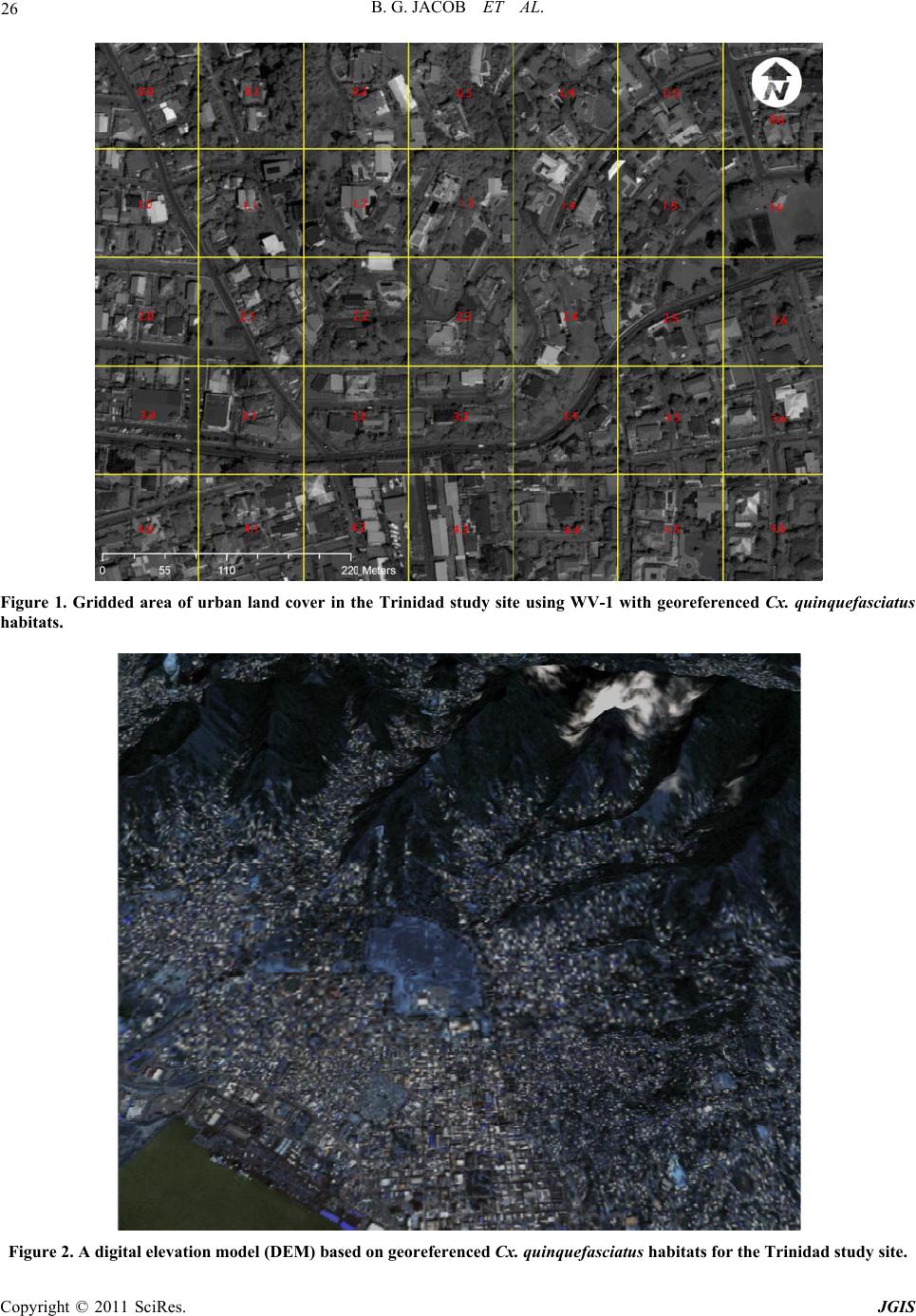

B. G. JACOB ET AL.
26
Figure 1. Gridded area of urban land cover in the Trinidad study site using WV-1 with georeferenced Cx. quinquefasciatus
habitats.
Figure 2. A digital elevation model (DEM) based on georeferenced Cx. quinquefasciatus habitats for the Trinidad study site.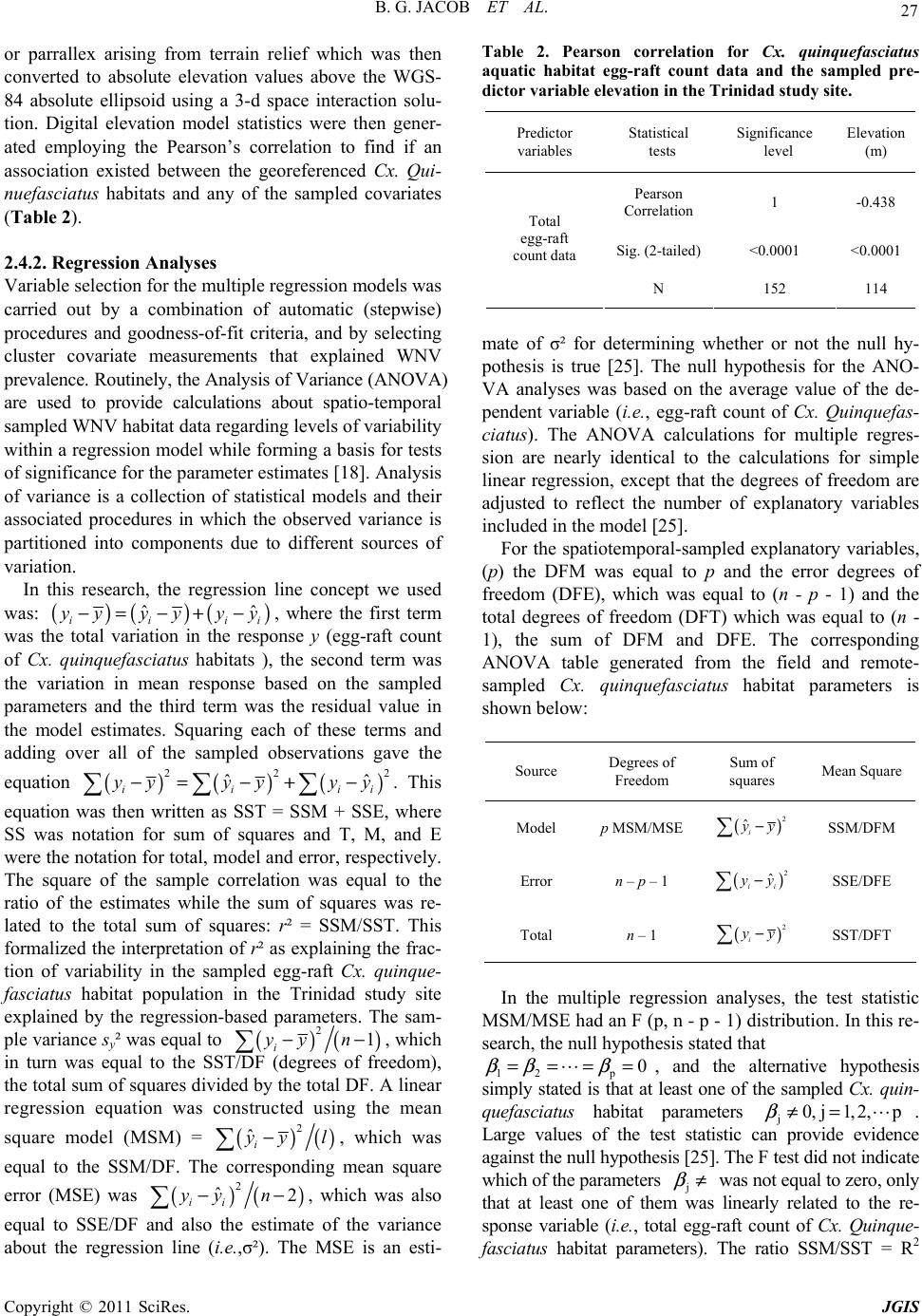

B. G. JACOB ET AL.
27
or parrallex arising from terrain relief which was then
converted to absolute elevation values above the WGS-
84 absolute ellipsoid using a 3-d space interaction solu-
tion. Digital elevation model statistics were then gener-
ated employing the Pearson’s correlation to find if an
association existed between the georeferenced Cx. Qui-
nue fa s ci a tus habitats and any of the sampled covariates
(Table 2).
2.4.2. Regression Analyses
Variable selection for the multiple regression models was
carried out by a combination of automatic (stepwise)
procedures and goodness-of-fit criteria, and by selecting
cluster covariate measurements that explained WNV
prevalence. Routinely, the Analysis of Variance (ANOVA)
are used to provide calculations about spatio-temporal
sampled WNV habitat data regarding levels of variability
within a regression model while forming a basis for tests
of significance for the parameter estimates [18]. Analysis
of variance is a collection of statistical models and their
associated procedures in which the observed variance is
partitioned into components due to different sources of
variation.
In this research, the regression line concept we used
was:
()()( )
ˆˆ
iiii
y
yyyyy−=−+ − , where the first term
was the total variation in the response y (egg-raft count
of Cx. quinquefasciatus habitats ), the second term was
the variation in mean response based on the sampled
parameters and the third term was the residual value in
the model estimates. Squaring each of these terms and
adding over all of the sampled observations gave the
equation
()()( )
22 2
ˆˆ
iiii
yyyy yy−=−+ −

. This
equation was then written as SST = SSM + SSE, where
SS was notation for sum of squares and T, M, and E
were the notation for total, model and error, respectively.
The square of the sample correlation was equal to the
ratio of the estimates while the sum of squares was re-
lated to the total sum of squares: r² = SSM/SST. This
formalized the interpretation of r² as explaining the frac-
tion of variability in the sampled egg-raft Cx. quinque-
fasciatus habitat population in the Trinidad study site
explained by the regression-based parameters. The sam-
ple variance sy² was equal to
() ()
21
i
yy n−−
, which
in turn was equal to the SST/DF (degrees of freedom),
the total sum of squares divided by the total DF. A linear
regression equation was constructed using the mean
square model (MSM) =
() ()
2
ˆi
yy l−
, which was
equal to the SSM/DF. The corresponding mean square
error (MSE) was
() ()
2
ˆ2
ii
yy n−−
, which was also
equal to SSE/DF and also the estimate of the variance
about the regression line (i.e.,σ²). The MSE is an esti-
Table 2. Pearson correlation for Cx. quinquefasciatus
aquatic habitat egg-raft count data and the sampled pre-
dictor variable elevation in the Trinidad study site.
Predictor
variables
Statistical
tests
Significance
level
Elevation
(m)
Pearson
Correlation 1 -0.438
Sig. (2-tailed) <0.0001 <0.0001
Total
egg-raft
count data
N 152 114
mate of σ² for determining whether or not the null hy-
pothesis is true [25]. The null hypothesis for the ANO-
VA analyses was based on the average value of the de-
pendent variable (i.e., egg-raft count of Cx. Quinquefas-
ciatus). The ANOVA calculations for multiple regres-
sion are nearly identical to the calculations for simple
linear regression, except that the degrees of freedom are
adjusted to reflect the number of explanatory variables
included in the model [25].
For the spatiotemporal-sampled explanatory variables,
(p) the DFM was equal to p and the error degrees of
freedom (DFE), which was equal to (n - p - 1) and the
total degrees of freedom (DFT) which was equal to (n -
1), the sum of DFM and DFE. The corresponding
ANOVA table generated from the field and remote-
sampled Cx. quinquefasciatus habitat parameters is
shown below:
Source Degrees of
Freedom
Sum of
squares Mean Square
Model p MSM/MSE ()
2
ˆi
yy−
 SSM/DFM
Error n – p – 1
()
2
ˆ
ii
yy−
 SSE/DFE
Total n – 1
()
2
i
yy−
 SST/DFT
In the multiple regression analyses, the test statistic
MSM/MSE had an F (p, n - p - 1) distribution. In this re-
search, the null hypothesis stated that
12p
0
ββ β
====, and the alternative hypothesis
simply stated is that at least one of the sampled Cx. quin-
quefasciatus habitat parameters j0,j1, 2,p
β
≠=.
Large values of the test statistic can provide evidence
against the null hypothesis [25]. The F test did not indicate
which of the parameters j
β
≠ was not equal to zero, only
that at least one of them was linearly related to the re-
sponse variable (i.e., total egg-raft count of Cx. Quinque-
fasciatus habitat parameters). The ratio SSM/SST = R2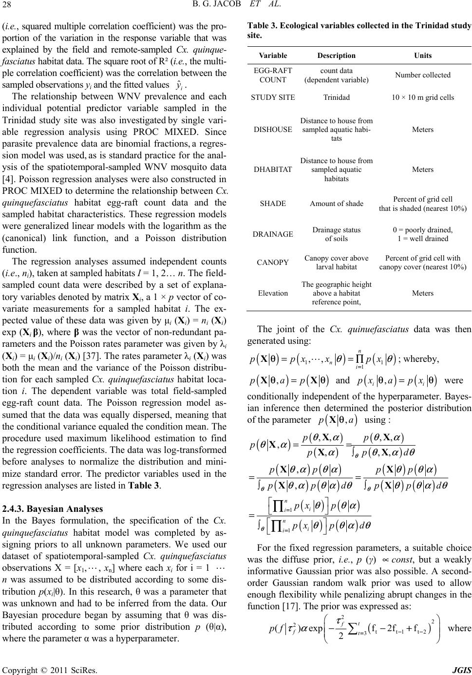

B. G. JACOB ET AL.
28
(i.e., squared multiple correlation coefficient) was the pro-
portion of the variation in the response variable that was
explained by the field and remote-sampled Cx. quinque-
fasciatus habitat data. The square root of R² (i.e., the multi-
ple correlation coefficient) was the correlation between the
sampled observations yi and the fitted values ˆi y.
The relationship between WNV prevalence and each
individual potential predictor variable sampled in the
Trinidad study site was also investigated by single vari-
able regression analysis using PROC MIXED. Since
parasite prevalence data are binomial fractions, a regres-
sion model was used, as is standard practice for the anal-
ysis of the spatiotemporal-sampled WNV mosquito data
[4]. Poisson regression analyses were also constructed in
PROC MIXED to determine the relationship between Cx.
quinquefasciatus habitat egg-raft count data and the
sampled habitat characteristics. These regression models
were generalized linear models with the logarithm as the
(canonical) link function, and a Poisson distribution
function.
The regression analyses assumed independent counts
(i.e., ni), taken at sampled habitats I = 1, 2… n. The field-
sampled count data were described by a set of explana-
tory variables denoted by matrix Xi, a 1 × p vector of co-
variate measurements for a sampled habitat i. The ex-
pected value of these data was given by μi (Xi) = ni (Xi)
exp (Xi β), where β was the vector of non-redundant pa-
rameters and the Poisson rates parameter was given by λi
(Xi) = μi (Xi)/ni (Xi) [37]. The rates parameter λi (Xi) was
both the mean and the variance of the Poisson distribu-
tion for each sampled Cx. quinquefasciatus habitat loca-
tion i. The dependent variable was total field-sampled
egg-raft count data. The Poisson regression model as-
sumed that the data was equally dispersed, meaning that
the conditional variance equaled the condition mean. The
procedure used maximum likelihood estimation to find
the regression coefficients. The data was log-transformed
before analyses to normalize the distribution and mini-
mize standard error. The predictor variables used in the
regression analyses are listed in Table 3.
2.4.3. Bayesian Analyses
In the Bayes formulation, the specification of the Cx.
quinquefasciatus habitat model was completed by as-
signing priors to all unknown parameters. We used our
dataset of spatiotemporal-sampled Cx. quinquefasciatus
observations X = [x1,, xn] where each xi for i = 1 
n was assumed to be distributed according to some dis-
tribution p(xi|θ). In this research, θ was a parameter that
was unknown and had to be inferred from the data. Our
Bayesian procedure began by assuming that θ was dis-
tributed according to some prior distribution p (θ|α),
where the parameter α was a hyperparameter.
Table 3. Ecological variables collected in the Trinidad study
site.
Variable Description Units
EGG-RAFT
COUNT
count data
(dependent variable) Number collected
STUDY SITETrinidad 10 × 10 m grid cells
DISHOUSE
Distance to house from
sampled aquatic habi-
tats
Meters
DHABITAT
Distance to house from
sampled aquatic
habitats
Meters
SHADE Amount of shade Percent of grid cell
that is shaded (nearest 10%)
DRAINAGE Drainage status
of soils
0 = poorly drained,
1 = well drained
CANOPY Canopy cover above
larval habitat
Percent of grid cell with
canopy cover (nearest 10%)
Elevation
The geographic height
above a habitat
reference point,
Meters
The joint of the Cx. quinuefasciatus data was then
generated using:
()()()
11
1
,, n
ni
ppxx px θθ
=
θ= =∏X; whereby,
()()
,papθ= θXX and
()()
,
ii
px a pxθ= θ were
conditionally independent of the hyperparameter. Bayes-
ian inference then determined the posterior distribution
of the parameter
()
,paθX using :
()
()
()
()
()
()()
()() ()() ()()
()()
()()
1
1
,, ,,
,,,,
,
,
n
i
i
n
i
i
pp
pppd
pp pp
ppdppd
px p
px pd
θ
θθ
θ
θα θα
θα αθαθ
θα θαθ θα
θ αθαθθθαθ
θθα
θθαθ
=
=
==

==



=

∏
∏
XX
XXX
XX
XX
For the fixed regression parameters, a suitable choice
was the diffuse prior, i.e., p (γ) ∝const, but a weakly
informative Gaussian prior was also possible. A second-
order Gaussian random walk prior was used to allow
enough flexibility while penalizing abrupt changes in the
function [17]. The prior was expressed as:
()
22
2
tt1t2
3
()exp f2ff
2
t
f
ft
pf
τ
τα
−−
=
−−+




 where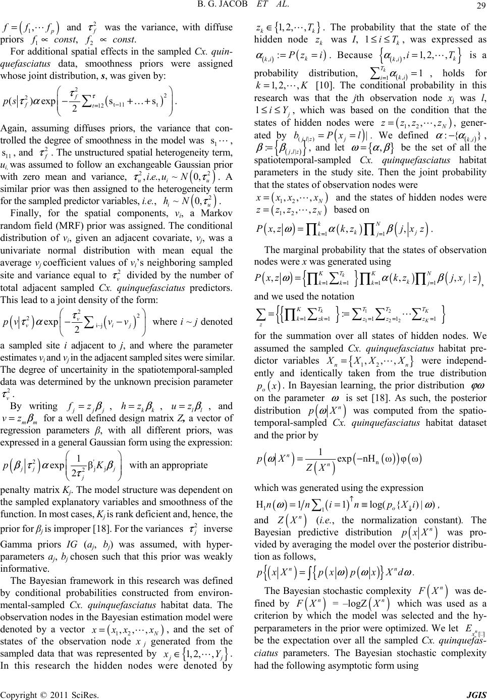

B. G. JACOB ET AL.
29
()
1,
p
f
ff= and 2
f
τ was the variance, with diffuse
priors 1
f
∝ const, 2
f
∝ const.
For additional spatial effects in the sampled Cx. quin-
que fa sc ia tu s data, smoothness priors were assigned
whose joint distribution, s, was given by:
()
22
2
t11 t
12
()exps s
2
f
ft
ps
τ
τ
τα
−
=

−+…+ 


.
Again, assuming diffuses priors, the variance that con-
trolled the degree of smoothness in the model was 1
s,
11
s, and 2
f
τ . The unstructured spatial heterogeneity term,
ui, was assumed to follow an exchangeable Gaussian prior
with zero mean and variance,
()
22
,.., ~0,
ui u
ie uN ττ . A
similar prior was then assigned to the heterogeneity term
for the sampled predictor variables, i.e. ,
()
2
~0,
iu
hN τ .
Finally, for the spatial components, vi, a Markov
random field (MRF) prior was assigned. The conditional
distribution of vi, given an adjacent covariate, vj, was a
univariate normal distribution with mean equal the
average vj coefficient values of vi’s neighboring sampled
site and variance equal to 2
v
τ divided by the number of
total adjacent sampled Cx. quinquefasciatus predictors.
This lead to a joint density of the form:
()
()
22
2
i~j
exp 2
v
vij
pvv v
τ
τα

−−


 where i ~ j denoted
a sampled site i adjacent to j, and where the parameter
estimates vi and vj in the adjacent sampled sites were similar.
The degree of uncertainity in the spatiotemporal-sampled
data was determined by the unknown precision parameter
2
v
τ .
By writing
j
jj
f
z
β
=, kk hz
β
=, ll uz
β
=, and
mm
vz
β
= for a well defined design matrix Z, a vector of
regression parameters β, with all different priors, was
expressed in a general Gaussian form using the expression:
()
2'
jj
2
1
exp β
2
j
jj
j
pK
β
τα
β
τ




with an appropriate
penalty matrix Kj. The model structure was dependent on
the sampled explanatory variables and smoothness of the
function. In most cases, Kj is rank deficient and, hence, the
prior for βj is improper [18]. For the variances 2
j
τ inverse
Gamma priors IG (aj, bj) was assumed, with hyper-
parameters aj, bj chosen such that this prior was weakly
informative.
The Bayesian framework in this research was defined
by conditional probabilities constructed from environ-
mental-sampled Cx. quinquefasciatus habitat data. The
observation nodes in the Bayesian estimation model were
denoted by a vector
()
12
,,,
N
x
xx x=, and the set of
states of the observation node x j
generated from the
sampled data that was represented by
{
}
1, 2,,
j
j
x
Y∈.
In this research the hidden nodes were denoted by
{
}
1, 2,,
kk
zT∈. The probability that the state of the
hidden node k z was I, 1k iT≤≤ , was expressed as
()
()
,:k
ki
P
zi α == . Because
()
{
}
,,1,2,,
k
ki iT
α = is a
probability distribution,
()
,
11
k
T
ki
i
α
==
, holds for
1, 2,,kK= [10]. The conditional probability in this
research was that the jth observation node xj was l,
1
j
iY≤≤ , which was based on the condition that the
states of hidden nodes were
()
12
,, ,
N
zzz z=, gener-
ated by
()
(,|) | jlz j
bPxl==. We defined
()
,
:{ }
ki
αα −,
()
{
}
,|
:jlz ββ =, and let
{
}
, ωα
β
= be the set of all the
spatiotemporal-sampled Cx. quinquefasciatus habitat
parameters in the study site. Then the joint probability
that the states of observation nodes were
()
12
,,,
N
x
xx x= and the states of hidden nodes were
()
12
,, ,
N
zzz z= based on
()
()
()
11
,,,
kN
kj
kj
Pxzkz jxz ωα β
==
=∏∏ .
The marginal probability that the states of observation
nodes were x was generated using
()
{
}
()
()
1
11 1
,,,|
k
KK N T
kj
k
kk j
Pxzkzjx z ωαβ
=
== =
=
∏∏ ∏,
and we used the notation
{
}
{
}
12
122
1111 1:
kK
K
KTTTT
zkz zz k
z
==== =
==
 ∏ 
for the summation over all states of hidden nodes. We
assumed the sampled Cx. quinquefasciatus habitat pre-
dictor variables
{
}
12
,,,
nn
X
XX X= were independ-
ently and identically taken from the true distribution
()
o
px
. In Bayesian learning, the prior distribution
ϕ
ω
on the parameter
ω is set [18]. As such, the posterior
distribution
()
n
pX ω was computed from the spatio-
temporal-sampled Cx. quinquefasciatus habitat dataset
and the prior by
()
()
()
()
()
n
1expnH ωφω
n
n
pX ZX ω =−
which was generated using the expression
() ()
11
H11log({) |)
o
nninpXi ωω
↑
↓
==≡
,
and
()
n
Z
X (i.e., the normalization constant). The
Bayesian predictive distribution
()
n
pxX was pro-
vided by averaging the model over the posterior distribu-
tion as follows,
()
{
()()
{
}
nn
pxXpx p xXd ωω ω =.
The Bayesian stochastic complexity
()
n
F
X was de-
fined by
()
n
F
X = –logZ
()
n
X
which was used as a
criterion by which the model was selected and the hy-
perparameters in the prior were optimized. We let []
n
x
E

be the expectation over all the sampled Cx. quinquefas-
ciatus parameters. The Bayesian stochastic complexity
had the following asymptotic form using

B. G. JACOB ET AL.
30
()()
() ()
[log1log log log1EXnFXnn mnO λ
↑↑
↓≈−− +
where λ and m were the rational number and the natural
number respectively, and the two were determined by the
singularities of sampled predictor variables. In regular
models, 2λ is equal to the number of parameters and m =
1, while in non-identifiable models, 2λ is not larger than
the number of parameters and m ≥ 1 [38]. However,
Bayesian frameworks using field and remote-sampled
vector mosquito data requires integration over the poste-
rior distribution, which typically cannot be performed
analytically [4].
In this research, we let
{
}
,
nn
X
Z be the sampled Cx.
quinuqefasciatus parameter estimates corresponding to
the hidden error variables in the equation n
Z
=
{
}
12
,,,
n
Z
ZZ. The variational Bayesian framework
approximated the Bayesian posterior
()
,
nn
pZ X ω of
the hidden variables and the Cx. quinuqefasciatus pa-
rameters using the variational posterior
()
,
nn
qZ X ω ,
which was factorized using
()
()
()
,
nn nn n
qZXQZ XrX ωω =,
where
()
nn
QZ X and
()
n
rX ω were posteriors
based on the inconspicuous error variables and the sam-
pled data respectively. The variational posterior
()
,
nn
qZ X ω was chosen to minimize the functional
F
[q] defined by
[]
()()()
()
()
,log,
,,
n
nnnn n
nn
Z
qZ XqZ XpoX
qd
pX
FZ
ωω
ω
ω
=,
which was then further defined by the equation
()( )
()
(,|)||,|
s
FXnKqZnXnpZn Xn ωω
↑↑↑↑↑
=+
using the sampled parameters, where
()() ()
,| ||,|
K
qZnXnpZn Xn ωω
↑↑ ↑↑
and the true Bay-
esian posterior was
()
,|
nn
pZ X ω and the variational
posterior was
()
,
nn
qZ X ω . This led to the functional
[
]
F
q being minimized under the constraint and then the
variation posteriors,
()
n
rX ω , and
()
nn
QZ X which
was computed using the equations
()
()
()
1exp
nnn
r
rXlogpXZ Q
C
ωϕωω =< > and
()
()
1exp ,
nn nn
Q
Q ZXlogpXZr
C
ω =< >
where r
C and Q
C were the normalization constants. It
is important to note that these equations gave only nec-
essary conditions for the functional
[
]
F
q to be mini-
mized in the Cx. quinuqefasciatus habitat model. The
variational posteriors were computed by an iterative al-
gorithm. We defined the variational stochastic complex-
ity
()
n
F
X
by the minimum value of the functional
[
]
F
q which was
() []
min
r,Q
n
F
X
Fq=, based on the dif-
ference between
()
n
F
X
and the Bayesian stochastic
complexity
()
n
F
X.
We then generated variational posterior for the esti-
mation matrix. We assumed that the prior distribution
()
ϕ
ω of the Cx. quinquefasciatus habitat parameters
{
}
,ab ω = was the conjugate prior distribution. Then
()
ϕ
ω was generated by the equation
() ()
()
()
01
0
1,
0
Γ,1,2,,
Γ
k
kkk
T
k
kTzkz
T
aakK
φ
φ
ϕφ
−
=
==
∏,
and covariates estimates were provided by
()
()
()
()
0
0ξ1
(|) 1
0
Γξ ,1,2,,
Γξ
j
nnjj
jY
jz jzYx
Y
bbjN ϕ
−
=
==
∏,
which were Dirichlet distributions with hyperparame-
ters generated using 0
φ
> 0 and 0 ξ > 0. The Dirichlet
distribution [i.e., Dir(α)] is a family of continuous multi-
variate probability distributions parameterized by the
vector α of positive reals which can generate the multi-
variate generalization of the beta distribution and conju-
gate prior of the categorical distribution and multinomial
distribution in Bayesian statistics for predictive vector
mosquito habitat models [4]. The Dirichlet distribution is
the multinomial extension to the beta distribution for a
binomial process which can also be used in quantifying
probabilities in predictive vector mosquito habitat prob-
ability models [39].
We then let
()
n δ be 1 when n = 0 and 1 otherwise,
and then defined the sampled parameter uncertainty es-
timates using
()
()
()
()
,1
:
k
nk
z
ik
kz iQ
nZz δ
=
=−
. In this re-
search we also used
()
()
()
()
()
()
()
11
,:
j
K njk
x
ij ik
ik
jx zQ
nXxZz δδ
==
−=−
∏
.
In these equations,
()
j
i
X
was the state of the jth ob-
servation node and
()
k
i
Z
was the state of the kth hidden
node. The variational posterior distribution of parameters
{
}
,ab ω = was given by using the equation
()
()
()
()
()
0
k
,1
0
,
1
z
0
k,z
1
Γ(n )
|
Γn
x
kk
k
k k
k
Tnkz
nk
kkz
z T
z
T
ra Xa
φ
φ
φ
+−
=
=
+
=+∏
∏
where each of the spatiotemporal-sampled Cx. Quinqe-
fasciatus habitat covariates were generated using the
equation
() ()
() ()
()
()
()
:1
1
nzxi n
kKZikZkQ
↑
↑
↓↓
↑
↓↓↓
↓
==≡
=≡ −

∏

B. G. JACOB ET AL.
31
It then followed that 1(, |)
j
j
j
x
y
x
z
zj
xx
nn
=
= for 1,,jN=
and
() ,kk
z
x
z
kz z
nn
−
= denoted the sum over
()
i
zi k≠.
In this research we evaluated the statistical efficiency
of the MCMC sequence in WinBUGS® using the fol-
lowing steps:
Step1: Sample S(m) from f(S|X,Z(m-1))
Step2: Sample P(m) from f(P|X,S(m),Z(m-1))
Step3: Sample Z(m) from f(Z|X,P(m),S(m),Φ(m-1))
where X was the field and remote-sampled Cx. Quinque-
fasciatus habitat data and Z was randomly assigned a
starting value Z(1) using a uniform prior distribution.
Step 1 was performed by drawing from an inverse
Wishart distribution. In Bayesian statistics inverse Wi-
shart distribution is used as the conjugate prior for the
covariance matrix of a multivariate normal distribution
[9]. The probability density function of the inverse Wi-
shart was:
()
()
1
ψB/2
12
/2
2
ψ|||
22
trace
mp
m
mp
p
Be
m
τ
−
−
−++



where B and ψ were positive definite matrices, and
p
τ (·) was the multivariate gamma function. In this re-
search the distribution of the inverse of a Wishart-distrib-
uted matrix was generated from
()
~,
A
Wm
 and
, which was of size of the matrix constructed from
the field and remote-sampled Cx. quinquefasciatus habi-
tat parameters. Under these circumstances 1 BA
−
= had
an inverse Wishart distribution,
()
1
1
~,BWm
−
−. We
calculated the probability density function:
()
()
1
/2 1
2
2
|||exptrB 2
|,
22
mp
m
mp
p
B
pB mm
ψψ
ψ
τ
++
−−
−
=


where 1 ψ
−
=and
p
τ
(·) was the multivariate gamma
function of the sampled data. A probability density func-
tion or density of a continuous random variable is a func-
tion that describes the relative likelihood for this random
variable to occur at a given point [25].
The marginal and conditional distributions from the
inverse Wishart-distributed matrix was quantified using
()
1
~,
A
Wm ψ
−. We then partitioned the matrices for
determining if
ψ
was conformable with each other
using:
11 12
21 22
AA
AAA

=

, 11 12
21 22
ψψ
ψψψ

=

where Aij and ij
ψ
were Pi x Pj matrices. We then
determined if:
1) 11 A was independent of 1
11 12
AA
− and 221
A⋅, when
1
22 122211112
AAAAA
−
⋅=− which was the Schur com-
plement (i.e., a submatrix within a larger matrix) of 11 A
in A;
2) 11 A~
()
1
11 2
,Wmp ψ
−−;
3) 12
111
111222 1x111222 111
AA |A~(,A)
pp
MN ψψψ
−−−
⋅⋅
⊗ ,
where (,)
pxq
MN ⋅⋅ was a matrix normal distribution gen-
erated from the spatiotemporal-sampled Cx. quinque-
fasciatus habitat parameters;
4)
()
1
22 111
A~ ,Wm ψ
−
⋅.
We used the Conjugate distribution to make inference
about a covariance matrix whose prior
()
p

had a
()
1
11,Wm
ψ
− distribution. If the observations
1,, n
X
xx= are independent p-variate Gaussian vari-
ables drawn from a
()
0,N

distribution, then the con-
ditional distribution p

X has a
()
1,Wnm
ψ
−++A
distribution, where A =XXT is n times the sample co-
variance matrix [3]. Because the prior and posterior dis-
tributions are the same family, the inverse Wishart dis-
tribution was the conjugate to the multivariate Gaussian
generated from the georeferenced Cx. quinquefasciatus
habitat parameters.
Due to its conjugacy to the multivariate Gaussian it
was possible to “integrate out” the Gaussian’s parameter

using:
() ()()
2
22
X, X,
2
A2
m
p
np mn
p
PmPPmd
mn
m
ψψ
ψτ
πψτ
+
=
+



=
+

 

This task was simplified by assuming that the spatio-
temporal-sampled Cx. quinquefasciatus habitat data
analyses had covariance matrices with common eigen-
vectors. If covariance’s differ among sources, the inverse
Wishart draws often produce invalid, especially for
sources that are small components of the mixture [9]. In
this research we developed a different approach, noting
that a covariance matrix S can be decomposed into a
vector of standard deviations, V, and a correlation matrix,
R using: S = diag(V)Rdiag(V) where diag(V) was a ma-
trix with diagonal elements V and zeros elsewhere. This
decomposition permitted the independent sampling of V
and R. We simulated the standard deviations, V, from an
inverse gamma distribution:
()
()
2
1,
2
,,~ ,
22
mklk
k
kl
s
n
n
pV XZIG αβ
−
++



, where nk
was the number of individual habitats assigned to cluster
k by Z(m-1) (i.e., an estimate of the Cx. quinquefasciatus
habitat sample size), s2
k,l was the sample variance of

B. G. JACOB ET AL.
32
element l in cluster k as assigned by Z(m-1), and α and β
were constants, both set to the non-informative prior
value of 1. Quasi-likelihood techniques in a logistic re-
gression equation and Bayesian prior distributions can
enumerate intra-cluster correlations in urban vector
mosquito aquatic habitats [4].
We simulated the elements of the correlation matrices,
R, from a hyperbolic-tangent transformed distribution
using :
()
()
() () ()
1
,, ,,
1
tanh|,~ˆ tanh ,
m
ki jki j
k
pRXRZN n
−
where ,,
ˆki j
R was the current estimate of the correlation
between the ith and jth elements (i ≠ j) in a cluster k given
Z(m-1), and nk was the same. After sampling values for
both V and R, we reassembled the covariance matrix, Sk,
for each Cx. quinquefasciatus habitat cluster, thus, com-
pleting Step 1.
Step 2 required drawing values for the elemental
means, P. The field and remote-sampled data X had an
approximate multivariate normal distribution as such
Step 2 was performed using the vector of mean concen-
trations for cluster k. The multivariate normal distribu-
tion using the Cx. quinquefasciatus habitat parameters
was given by the sample means calculated from X, gen-
erated from the cluster assignments, Z(m-1)) and the co-
variance Sk from Step 1. If cluster k was empty at m-1
(that was, no individual sampled habitat parameters were
assigned to k by Z(m-1)), then the grand mean and covari-
ance matrix of X were used as the sample mean and co-
variance matrix of k.
Step 3 involved drawing new cluster assignments us-
ing each individual sampled Cx. quinquefasciatus habitat
in the Trinidad study site. To do so, it was necessary to
calculate Pr(zi = k) for every i, k combination (zi was the
ith element of Z). Again we assumed multivariate normal
distributions where Z(m) was simulated from:
()() ()
()
() ()
()
()()
()
,
1
Pr| ,,,
|,,
|,,
kk
immm
mm
ii
kkk
Kmm
ii
k
K
zkXPS
fX PSzk
f
XPSz k
φ
φ
φ
′′
′
−
=
=
=′
=

and where the
()
f⋅ terms on the right-hand side were
multivariate normal likelihoods. Thus, the likelihood that
the ith element of X was present in the Cx. Quinquefas-
ciatus habitat population k, sampled in the study site
normalized by the sum of likelihoods was quantified for
all potential sources influencing presence of immatures.
Finally, the sample Φ(m) from f(Z|X, P(m), S(m), Z(m)) was
used to generate asymptotically efficient estimates from
the spatiotemporal-sampled data.
2.6. Eigenvector Mapping
We conducted a residual analyses using a misspecification
perspective for the error estimation models generated in
SAS/GIS® assuming that the basic regression model
*
yX
β
ε =+ had autocorrelated disturbances * ε , which
was decomposed into a white-noise component,
ε , and a
set of unspecified and/or misspecified models that
had the structure
*
yXBE
ε
γ
ε
=
=++
 . In this research,
the misspecification term was E
γ
. Quantification of
topographic patterns generated from the distribution of
the georeferenced Cx. quinquefasciatus habitat covari-
ates was required to describe independent key dimen-
sions and underlying spatial processes for defining a pat-
tern in the misspecification term. This was accomplished
by expanding the matrix term:
()
1
0
kk
k
I
VV ρρ
−∞
=
−=
, as an infinite power series,
which was feasible under the assumption that the under-
lying spatial process in the data was stationary; note that
in this research 00 V ρ gave the identity matrix
I
. The
simultaneous autoregressive error model was then re-
written asyVyX VX
ρβρβ
ε −=− +
. Substituting these
transformation gave:
() ()
1
yIV XVX
ρβρβ
ε
−
=−− +




()
0
kk
k
yVXVX
ρβρβ
ε
∞
=
=−+

()
11
000
kkkkkk
kk k
yVXVX V
ρβρβ ρ
ε
∞∞ ∞
++
== =
=−+
 
()
110
0
1
kk kkkk
kkk
kk
k
misspecification term
yX VXVXV
yX V
βρ βρβρ
ε
βρεε
∞∞∞
== =
=
∞
=
⋅
=+ −+
=+ +
 


 
The misspecification term
()
1, ,
kk
Vk ρε =∞
 re-
mained uncorrelated with the exogenous variable,
X
, as
the standard OLS assumption of the disturbances, ε ,
were uncorrelated with the predictor variables generated
from the model. The spatial lag model was expressed as:
()
IVyX
ρβ
ε −=+. Substituting the transformation
gave:
()
()
0
1
kk
k
kk
k
misspecification term
yVX
yX VX
ρβε
βρ β
εε
∞
=
∞
=
⋅
=+
=+ ++



The misspecification term
()( )
1, ,
kk
VX k ρβε +=∞

 included the exogenous

B. G. JACOB ET AL.
33
variables
X
. Consequently, the exogenous variables
were correlated with the misspecification term. Under
this condition, standard OLS results for the basic regres-
sion model* yX
β
ε =+, generated from the spatiotem-
poral-sampled covariates provided biased estimates ˆ
β
of the underlying regression parameters
β
.
The correlation, or lack thereof, between the exoge-
nous variables and the misspecification terms of both
habitat models were used to design spatial proxy vari-
ables, so that the properties of either model could be sat-
isfied. We considered two different projection matrices.
Different sets of eigenvectors were established using a
spatial regression model. This model feature enabled us
to also use the eigenvector spatial filtering approach for
predictions of the endogenous variable y.
We selected an evaluation criterion using the stan-
dardized Moran’s statistic. The standardized Moran’s
coefficient (MC) for regression residuals *
ˆ
ε was de-
fined as
() ()
()
2
iiji j
j
iij
ji
i
wXX XX
N
IwXX
−−
=−

 , where N
was the number of sampled habitats and their respective
parameter estimates indexed by i and j respectively; X
was the spatiotemporal-sampled egg-raft count data;
X
was the mean of X; and wij was a matrix of spatial
weights. The expected value of Moran’s I under hy-
pothesis of no spatial autocorrelation was:
()
1
1
EI N
−
=−. Its variance equaled:
() ()( )()
()
435
2
12 3
iij
j
NSS S
Var I
NN Nw
−
=
−− −
 where
()
()
()
()
()
() ()
()
2
1
2
2
4
1
32
2
1
2
2
12
4
2
51 1
1
2
1
33 3
1
6
21
ij ji
ij
ij ji
ij j
i
i
i
i
iij
j
iij
j
Sww
ww
S
Nxx
S
Nxx
NNSNS w
S
w
SS NS
−
−
=+
+
=
−
=
−
−+− +
=
=− +

 




In this research, negative (positive) values indicated
negative (positive) spatial autocorrelation. Values ranged
from -1 (indicating perfect dispersion) to +1 (perfect
correlation). A zero values indicated a random spatial
pattern. For statistical hypothesis testing predictive WNV
mosquito habitat modeling, MC values can be trans-
formed to z-scores in which values greater than 1.96 or
smaller than −1.96 indicate spatial autocorrelation that is
significant at the 5% level [8,29].
Geary’s Contiguity Ratio (GC) another measure of
spatial autocorrelation was also generated. GC is in-
versely related to the Moran’s statistic but it is not iden-
tical. Moran's indices are measure of global spatial auto-
correlation, while Geary’s C is more sensitive to local
spatial autocorrelation in vector mosquito data analyses
[16]. In this research, the sampled Cx. quinquefasciatus
habitat data was quantified by GC which was defined as
()
()
()
2
2
1
2
iijij
j
i
i
NwXX
C
WXX
−−
=−

 where N was the
number of the sampled habitats and explanatory parame-
ters indexed by i and j respectively; X was the egg-raft
count data;
X
was the mean of X; wij was a matrix of
spatial weights; and W was the sum of all wij. The value
of GC lies between 0 and 2. 1 means no spatial autocor-
relation while 0 refers to a chaotic random distribution.
Smaller (larger) than 1 means positive (negative) spatial
autocorrelation [8].
In this research, distance between sampled habitats
was defined in terms of an n-by-n geographic weights
matrix, C, whose cij values were; 1 if the sampled Cx.
quinquefasciatus egg-raft count locations i and j in the
Trinidad study site were deemed nearby, and 0 other-
wise. Adjusting this matrix by dividing each row entry
by its row sum gave C1, where 1 was an n-by-1 vector
of one’s which converted this matrix to matrix W. The
resulting autoregressive model specification with no
sampled covariates present (i.e., the pure spatial auto-
regression specification) took on the following form:
()
μ1-ρρ =++Y1WYε (2.1), where μ was the scalar
conditional mean of Y and ε was an n-by-1 error vec-
tor residuals of the sampled data which in this research
was represented as statistically independent and identi-
cally distributed (iid) normally random variates. The
spatial covariance matrix for equation (2.1), using the
sampled covariates, was
()()()()
12
E-μ'-μ- ρ'- ρσ
−
==  
 
Y1 Y1ΣIWIW ,
where E (⋅) indicated the calculus of expectations, I was
the n-by-n identity matrix denoting the matrix transpose
operation, and 2
σ was the error variance.
Two different autoregressive parameters appeared in
the spatial covariance matrix. When autocorrelation is
present in residual data, a more explicit representation of
both effects leads to a more accurate interpretation of
empirical results [38]. Consequently, we used an SAR
model specification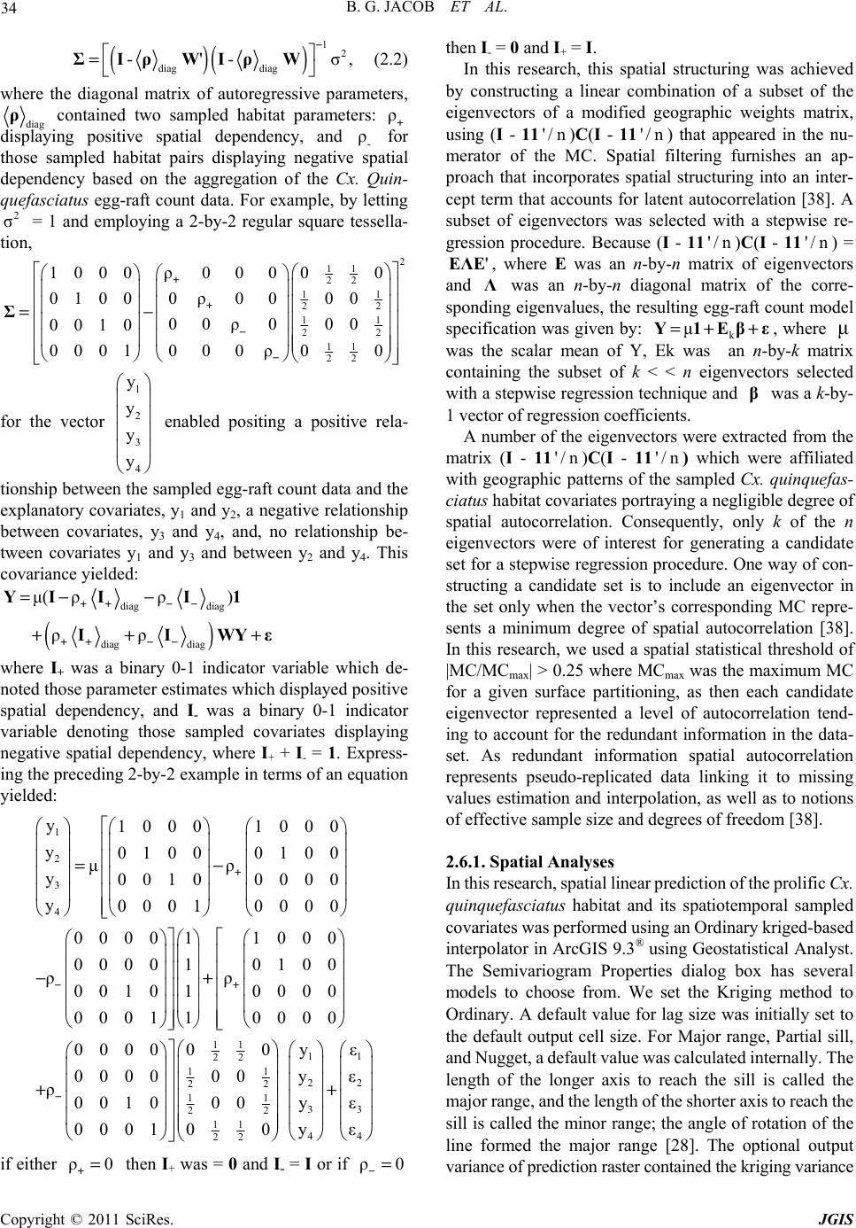

B. G. JACOB ET AL.
34
()()
12
diag diag
- '- σ,
−

= ΣIρWIρW (2.2)
where the diagonal matrix of autoregressive parameters,
diag
ρ contained two sampled habitat parameters: ρ+
displaying positive spatial dependency, and -
ρ for
those sampled habitat pairs displaying negative spatial
dependency based on the aggregation of the Cx. Quin-
quefasciatus egg-raft count data. For example, by letting
2
σ = 1 and employing a 2-by-2 regular square tessella-
tion,
2
11
22
11
22
11
22
11
22
00ρ000 1000
000ρ00 0100
0000ρ0 0010
00000ρ 0001
+
+
−
−


 
 
 
 


=−
 
 


  

 


Σ
for the vector
1
2
3
4
y
y
y
y






enabled positing a positive rela-
tionship between the sampled egg-raft count data and the
explanatory covariates, y1 and y2, a negative relationship
between covariates, y3 and y4, and, no relationship be-
tween covariates y1 and y3 and between y2 and y4. This
covariance yielded:
()
diag diag
diag diag
μ(ρ ρ)
ρ ρ
++ −−
++ −−
=− −
++ +
YI II1
IIWYε
where I+ was a binary 0-1 indicator variable which de-
noted those parameter estimates which displayed positive
spatial dependency, and I- was a binary 0-1 indicator
variable denoting those sampled covariates displaying
negative spatial dependency, where I+ + I- = 1. Express-
ing the preceding 2-by-2 example in terms of an equation
yielded:
1
2
3
4
y1000 1000
y0100 0100
μρ
y0010 0000
y00010000
000011000
000010100
ρρ
001010000
000110000
0000
0000
ρ0010
0001
+
−+
−

 
  
  
=−
  
  

 




 
−+
 






+
11 11
22
11
22
22
11
33
22
11 44
22
00yε
00y ε
00y ε
00yε

 



  +

 

 


 
 
if either ρ0
+= then I+ was = 0 and I- = I or if ρ0 −=
then I- = 0 and I+ = I.
In this research, this spatial structuring was achieved
by constructing a linear combination of a subset of the
eigenvectors of a modified geographic weights matrix,
using (I - 11 '/n)C(I - 11 '/n) that appeared in the nu-
merator of the MC. Spatial filtering furnishes an ap-
proach that incorporates spatial structuring into an inter-
cept term that accounts for latent autocorrelation [38]. A
subset of eigenvectors was selected with a stepwise re-
gression procedure. Because (I - 11 '/n)C(I - 11 '/n) =
'EΛE, where E was an n-by-n matrix of eigenvectors
and Λ was an n-by-n diagonal matrix of the corre-
sponding eigenvalues, the resulting egg-raft count model
specification was given by: k
μ =+ +Y1Eβε, where μ
was the scalar mean of Y, Ek was an n-by-k matrix
containing the subset of k < < n eigenvectors selected
with a stepwise regression technique and β was a k-by-
1 vector of regression coefficients.
A number of the eigenvectors were extracted from the
matrix (I - 11'/n)C(I - 11 '/n) which were affiliated
with geographic patterns of the sampled Cx. quinquefas-
ciatus habitat covariates portraying a negligible degree of
spatial autocorrelation. Consequently, only k of the n
eigenvectors were of interest for generating a candidate
set for a stepwise regression procedure. One way of con-
structing a candidate set is to include an eigenvector in
the set only when the vector’s corresponding MC repre-
sents a minimum degree of spatial autocorrelation [38].
In this research, we used a spatial statistical threshold of
|MC/MCmax| > 0.25 where MCmax was the maximum MC
for a given surface partitioning, as then each candidate
eigenvector represented a level of autocorrelation tend-
ing to account for the redundant information in the data-
set. As redundant information spatial autocorrelation
represents pseudo-replicated data linking it to missing
values estimation and interpolation, as well as to notions
of effective sample size and degrees of freedom [38].
2.6.1. Spatial Analyses
In this research, spatial linear prediction of the prolific Cx.
quinquefasciatus habitat and its spatiotemporal sampled
covariates was performed using an Ordinary kriged-based
interpolator in ArcGIS 9.3® using Geostatistical Analyst.
The Semivariogram Properties dialog box has several
models to choose from. We set the Kriging method to
Ordinary. A default value for lag size was initially set to
the default output cell size. For Major range, Partial sill,
and Nugget, a default value was calculated internally. The
length of the longer axis to reach the sill is called the
major range, and the length of the shorter axis to reach the
sill is called the minor range; the angle of rotation of the
line formed the major range [28]. The optional output
variance of prediction raster contained the kriging variance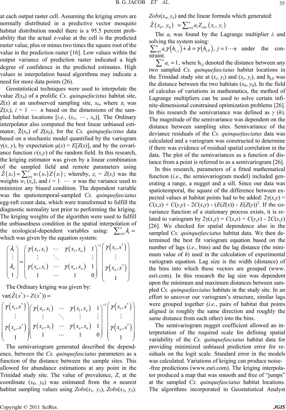

B. G. JACOB ET AL.
35
at each output raster cell. Assuming the kriging errors are
normally distributed in a predictive vector mosquito
habitat distribution model there is a 95.5 percent prob-
ability that the actual z-value at the cell is the predicted
raster value, plus or minus two times the square root of the
value in the prediction raster [16]. Low values within the
output variance of prediction raster indicated a high
degree of confidence in the predicted estimates. High
values in interpolation based algorithms may indicate a
need for more data points (26).
Geostatistical techniques were used to interpolate the
value Z(x0) of a prolific Cx. quinquefacistus habitat site,
Z(x) at an unobserved sampling site, x0, where zi was
Z(xi), i = 1  n based on the dimensions of the sam-
pled habitat locations [i.e., (x1, , xn)]. The Ordinary
interpolator also computed the best linear unbiased esti-
mator, Ž(xo) of Z(x0), for the Cx. quinquefacistus data
based on a stochastic model quantified by the variogram
γ(x, y), by expectation μ(x) = E[Z(x)], and by the covari-
ance function c(x,y) of the random field. In this research,
the kriging estimator was given by a linear combination
of the sampled field and remote parameters using
() ()()
1
ˆn
oioi
i
Z
xwxZx
=
=; whereby, zi = Z(xi) was the
weights wi (xo), and i = 1  n was the variance used to
minimize any biased condition. The dependent variable
was the spatiotemporal-sampled Cx. quinquefasciatus
egg-raft count data, which were transformed to fulfill the
diagnostic normality test prior to performing the kriging.
The kriging weights of the algorithm were used to fulfill
the unbiasedness condition in the spatial interpolation of
the ecological-dependent variables using: 1
n
i
i
λ
==

which was given by the equation system:
() ()
() ()
()
()
*
11
1111
*
1
,
,,1
,,1
,
1110
1
n
nnnn
n
x
x
xx xx
xx xx
x
x
γ
λγγ
λγγ γ
−

 

 


=

 









  


The Ordinary kriging was given by:
()
()
() ()
() ()
()
()
**
**
1
11
11 1
**
1
ˆ
var(() ())
,,
,,1
,,1
,,
110
11
n
nnn
nn
Zx Zx
x
xxx
xx xx
xxxx
x
xxx
γγ
γγ
γγ
γγ
−
−=
 

 

 

 

 


 
 

 


 


The semivariogram generated described the depend-
ence, between the Cx. quinquefasciatus parameters as a
function of the distance between the sample sites. This
allowed for abundance estimations at any point in the
Trinidad study site. The value of prevalence, Z, at the
coordinate (x0, y
0) was estimated from the n nearest
habitat sampling values using Zobs(x1, y1), Zobs(x2, y
2).
Zobs(xn, yn) and the linear formula which generated:
() ()
00 1
ˆ, ,
n
i obsii
i
Z
xyaZ xy
=
=
The ai was found by the Lagrange multiplier λ and
solving the system using:
() ()
,,0
1, 1
n
iij i
iahh jn
γλγ
=+= =
under the con-
straint.
1
n
i
a=
, where hi,j denoted the distance between any
two sampled Cx. quinquefasciatus habitat locations in
the Trinidad study site at (xi, yi) and (xj, yj), and hj,0 was
the distance between the two habitats (x0, y0). In the field
of calculus of variations in mathematics, the method of
Lagrange multipliers can be used to solve certain infi-
nite-dimensional constrained optimization problems [26].
In this research the semivariance was defined as γ (h).
The magnitude of the semivariance was dependent on the
distance between sampling sites. Semivariance of the
deviance residuals of the Cx. quinquefasciatus data was
calculated and a variogram was constructed to determine
if there was evidence of residual spatial correlation in the
data. The plot of the semivariances as a function of dis-
tance from a point is referred to as a semivariogram [26].
In this research, parameters of a fitted mathematical
function (i.e., the semiovariogram model) included gen-
erating a range, a nugget and a sill. Since our data was
spatiotemporal, the square of the difference between ex-
pected values at habitat points had to be added: 2γ(x,y) =
C(x,x) + C(y,y) - 2C(x,y) - (E(Z(x)) - E(Z(y))2. If the co-
variance function of a stationary process exists, it is re-
lated to variogram by 2γ(x,y) = C(x,x) + C(y,y) - 2C(x,y)
[26]. We checked for spatial dependence also in the
sampled Cx. quinquefasciatus habitat data. We then de-
termined the best fit variogram equation based on the
number of lags (i.e., bins) and the lag distance (the mini-
mum value of h) used in the calculation of experimental
variogram equation. Lag size is the width (distance) of
the bins into which these vectors are grouped (www.
esri.com). In this research the lag size was dependent
upon the minimum and maximum distances between sam-
pled Cx. quinquefasciatus habitats in the study site. In an
effort to uncover our variogram’s structure, similar lags
were grouped together (i.e., pairs of habitat that points
aligned in roughly the same direction and roughly the
same distance from each other) into the bins.
The semivariogram nugget coefficient allowed an in-
terpretation of the required scale for defining spatial
variability of the Cx. quinquefasciatus habitat data for
providing minimized unbiased prediction error for re-
siduals on the logit scale. Standard error in the models
was calculated. Variations of kriging can produce noise-
-free predictions (www.esri.com). The kriging interpola-
tor produced a map that was smooth and free of “jumps”
at the sampled Cx. quinquefasciatus habitat locations.
The algorithms incorporated in Geostatistical Analyst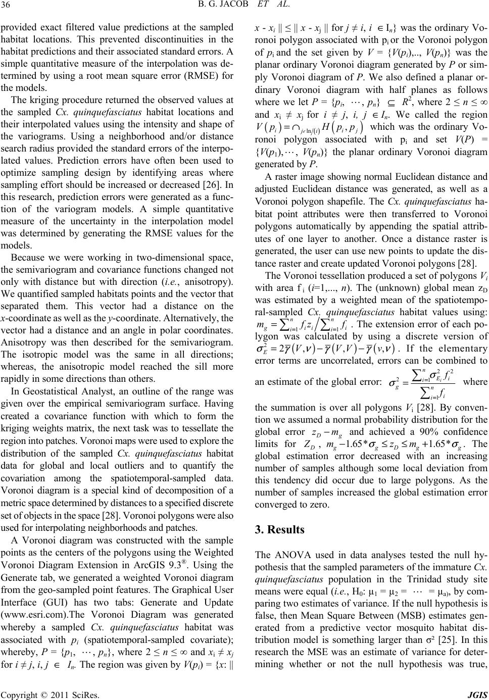

B. G. JACOB ET AL.
36
provided exact filtered value predictions at the sampled
habitat locations. This prevented discontinuities in the
habitat predictions and their associated standard errors. A
simple quantitative measure of the interpolation was de-
termined by using a root mean square error (RMSE) for
the models.
The kriging procedure returned the observed values at
the sampled Cx. quinquefasciatus habitat locations and
their interpolated values using the intensity and shape of
the variograms. Using a neighborhood and/or distance
search radius provided the standard errors of the interpo-
lated values. Prediction errors have often been used to
optimize sampling design by identifying areas where
sampling effort should be increased or decreased [26]. In
this research, prediction errors were generated as a func-
tion of the variogram models. A simple quantitative
measure of the uncertainty in the interpolation model
was determined by generating the RMSE values for the
models.
Because we were working in two-dimensional space,
the semivariogram and covariance functions changed not
only with distance but with direction (i.e. , anisotropy).
We quantified sampled habitats points and the vector that
separated them. This vector had a distance on the
x-coordinate as well as the y-coordinate. Alternatively, the
vector had a distance and an angle in polar coordinates.
Anisotropy was then described for the semivariogram.
The isotropic model was the same in all directions;
whereas, the anisotropic model reached the sill more
rapidly in some directions than others.
In Geostatistical Analyst, an outline of the range was
given over the empirical semivariogram surface. Having
created a covariance function with which to form the
kriging weights matrix, the next task was to tessellate the
region into patches. Voronoi maps were used to explore the
distribution of the sampled Cx. quinquefasciatus habitat
data for global and local outliers and to quantify the
covariation among the spatiotemporal-sampled data.
Voronoi diagram is a special kind of decomposition of a
metric space determined by distances to a specified discrete
set of objects in the space [28]. Voronoi polygons were also
used for interpolating neighborhoods and patches.
A Voronoi diagram was constructed with the sample
points as the centers of the polygons using the Weighted
Voronoi Diagram Extension in ArcGIS 9.3®. Using the
Generate tab, we generated a weighted Voronoi diagram
from the geo-sampled point features. The Graphical User
Interface (GUI) has two tabs: Generate and Update
(www.esri.com).The Voronoi Diagram was generated
whereby a sampled Cx. quinquefasciatus habitat was
associated with pi (spatiotemporal-sampled covariate);
whereby, P = {p1, , pn}, where 2 ≤ n ≤ ∞ and xi ≠ xj
for i ≠ j, i, j ∈ In. The region was given by V(pi) = {x: ||
x - xi || ≤ || x - xj || for j ≠ i, i ∈In} was the ordinary Vo-
ronoi polygon associated with pi or the Voronoi polygon
of pi and the set given by V = {V(pi),.., V(pn)} was the
planar ordinary Voronoi diagram generated by P or sim-
ply Voronoi diagram of P. We also defined a planar or-
dinary Voronoi diagram with half planes as follows
where we let P = {pi, , pn} ⊆ R2, where 2 ≤ n ≤ ∞
and xi ≠ xj for i ≠ j, i, j ∈In. We called the region
()
()
()
ln ,
iij ji
Vp Hpp=∩

which was the ordinary Vo-
ronoi polygon associated with pi and set V(P) =
{V(p1),, V(pn)} the planar ordinary Voronoi diagram
generated by P.
A raster image showing normal Euclidean distance and
adjusted Euclidean distance was generated, as well as a
Voronoi polygon shapefile. The Cx. quinquefasciatus ha-
bitat point attributes were then transferred to Voronoi
polygons automatically by appending the spatial attrib-
utes of one layer to another. Once a distance raster is
generated, the user can use new points to update the dis-
tance raster and create updated Voronoi polygons [28].
The Voronoi tessellation produced a set of polygons Vi
with area f i (i=1,..., n). The (unknown) global mean zD
was estimated by a weighted mean of the spatiotempo-
ral-sampled Cx. quinquefasciatus habitat values using:
11
n
gii
ii
n
i
mz
f
f
==
= . The extension error of each po-
lygon was calculated by using a discrete version of
()()()
22,, ,
EVVVv
σ
γ
ν
γγ
ν =−−. If the elementary
error terms are uncorrelated, errors can be combined to
an estimate of the global error:
22
21
1
i
n
E
i
i
gn
i
i
f
f
σ
σ
=
=
=
 where
the summation is over all polygons Vi [28]. By conven-
tion we assumed a normal probability distribution for the
global error
D
g
zm− and achieved a 90% confidence
limits for
D
Z
, 1.65* 1.65*
g
gD gg
mzm σσ −≤≤+ . The
global estimation error decreased with an increasing
number of samples although some local deviation from
this tendency did occur due to large polygons. As the
number of samples increased the global estimation error
converged to zero.
3. Results
The ANOVA used in data analyses tested the null hy-
pothesis that the sampled parameters of the immature Cx.
quinquefasciatus population in the Trinidad study site
means were equal (i.e., H0: µ1 = µ2 =  = µa), by com-
paring two estimates of variance. If the null hypothesis is
false, then Mean Square Between (MSB) estimates gen-
erated from a predictive vector mosquito habitat dis-
tribution model is something larger than σ² [25]. In this
research the MSE was an estimate of variance for deter-
mining whether or not the null hypothesis was true,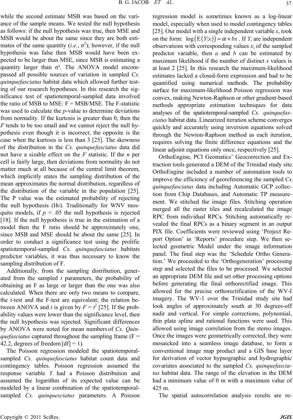

B. G. JACOB ET AL.
37
while the second estimate MSB was based on the vari-
ance of the sample means. We tested the null hypothesis
as follows: if the null hypothesis was true, then MSE and
MSB would be about the same since they are both esti-
mates of the same quantity (i.e., σ2); however, if the null
hypothesis was false then MSB would have been ex-
pected to be larger than MSE, since MSB is estimating a
quantity larger than σ². The ANOVA model encom-
passed all possible sources of variation in sampled Cx.
quinquefasciatus habitat data which allowed further test-
ing of our research hypotheses. In this research the sig-
nificance test of spatiotemporal-sampled data involved
the ratio of MSB to MSE: F = MSB/MSE. The F-statistic
was used to calculate the p-value to determine deviations
from normality. If the kurtosis is greater than 0, then the
F tends to be too small and we cannot reject the null hy-
pothesis even though it is incorrect; the opposite is the
case when the kurtosis is less than 3 [25]. The skewness
of the distribution in the Cx. quinquefasciatus data did
not have a sizable effect on the F statistic. If the n per
cell is fairly large, then deviations from normality do not
matter much at all because of the central limit theorem,
which implicitly states the sampling distribution of the
mean approximates the normal distribution, regardless of
the distribution of the variable in the population [25].
The P value was the estimated probability of rejecting
the null hypothesis (H0). Traditionally for WNV mos-
quito models, if p < .05 the null hypothesis is rejected
[18]. If the null hypothesis is true in the estimation of a
model then the F ratio should be approximately one,
since MSB and MSE should be about the same [25]. In
order to conduct a significance test using the prolific
spatiotemporal-sampled Cx. quinquefasciatus habitats
predictor variables, it was thus necessary to know the
sampling distribution of F.
Additionally, from the sampling distribution, gener-
ated from the sampled t parameters, the probability of
obtaining an F as large or larger than the one was also
calculated. When there are only two means to compare,
the t-test and the F-test are equivalent; the relation be-
tween ANOVA and t is given by F = t2 [25]. If the prob-
ability values were lower than the significance level, then
the null hypothesis was rejected. Significant differences
by ANOVA were noted for mean numbers of Cx. Quin-
quefasciatus captured throughout the sampling frame (F =
42.2, degrees of freedom [df] = 1).
The Poisson regression modeled the spatiotemporal-
sampled Cx. quinquefasciatus habitat count data and
contingency tables. Poisson regression assumed the
response variable Y had a Poisson distribution and
assumed the logarithm of its expected value can be
modeled by a linear combination of the spatiotemporal-
sampled Cx. quinquesciatus parameters. A Poisson
regression model is sometimes known as a log-linear
model, especially when used to model contingency tables
[25]. Our model with a single independent variable x, took
on the form:
() ()
log E|Yx bx α =+ . If Yi are independent
observations with corresponding values xi of the sampled
predictor variable, then a and b can be estimated by
maximum likelihood if the number of distinct x values is
at least 2 [25]. In this research the maximum-likelihood
estimates lacked a closed-form expression and had to be
quantified using numerical methods. The probability
surface for maximum-likelihood Poisson regression was
convex, making Newton-Raphson or other gradient-based
methods appropriate estimation techniques for data
analyses of the spatiotemporal-sampled Cx. quinquefas-
ciatus habitat data. Linearized iteration scheme converges
quickly and accurately using inversion equations solved
through the Newton-Raphson method as each iteration,
requires solving the finite difference equations and the
linear adjoint equations only once, respectively [25].
OrthoEngine, PCI Geomatics’ Geocorrection and Ex-
traction tools generated a DEM of the Trinidad study site.
OrthoEngine included a number of automation tools to
improve the efficiency of georeferencing the sampled Cx.
quinquefasciatus data including Automatic GCP collec-
tion from Chip Databases, and Automatic TP measure-
ment. We stitched the image files. Stitching operation
merged all the raster tiles and recalculated the image
RPC from individual RPCs. Stitching automatically re-
vealed the final RPCs as a binary segment in an output
PIX file. Coefficients were reviewed using ‘Project Re-
port Option’ in ‘Reports’ procedure step. We then se-
lected geometric Model under the image information
panel. The final step was the ‘Schedule Ortho Genera-
tion.’ We proceeded to the ‘Orthogeneration’ processing
step and selected the files to be processed. We selected
an appropriate DEM file and set other processing options
before generating the final orthorectified image. This
allowed for the precise orthorectification of the WV-I
imagery. The WV-1 over the Trinidad study site had
look angles of approximately south at 30 degrees-off
nadir and vertical. For simple corrections, polynomial,
thin plate spline and rational functions were used. This
allowed using image correlation from the stereo images.
Once the images were geometrically corrected, they were
mosaicked into a seamless image database, to form a
conventional image map product and a GIS base layer
for derivation of vector hypsographic and hydrographic
covariates associated to the sampled Cx. quinquefascia-
tus habitat data. The range of the elevation in the DEM
had a minimum value of 0 m with a maximum value of
425 m.
The spatial autocorrelation analysis results are re-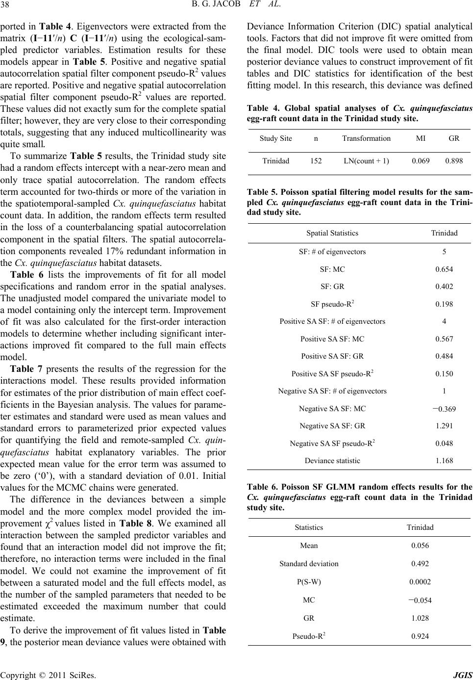

B. G. JACOB ET AL.
38
ported in Table 4. Eigenvectors were extracted from the
matrix (I−11′/n) C (I−11′/n) using the ecological-sam-
pled predictor variables. Estimation results for these
models appear in Table 5. Positive and negative spatial
autocorrelation spatial filter component pseudo-R2 values
are reported. Positive and negative spatial autocorrelation
spatial filter component pseudo-R2 values are reported.
These values did not exactly sum for the complete spatial
filter; however, they are very close to their corresponding
totals, suggesting that any induced multicollinearity was
quite small.
To summarize Table 5 results, the Trinidad study site
had a random effects intercept with a near-zero mean and
only trace spatial autocorrelation. The random effects
term accounted for two-thirds or more of the variation in
the spatiotemporal-sampled Cx. quinquefasciatus habitat
count data. In addition, the random effects term resulted
in the loss of a counterbalancing spatial autocorrelation
component in the spatial filters. The spatial autocorrela-
tion components revealed 17% redundant information in
the Cx. quinquefasciatus habitat datasets.
Table 6 lists the improvements of fit for all model
specifications and random error in the spatial analyses.
The unadjusted model compared the univariate model to
a model containing only the intercept term. Improvement
of fit was also calculated for the first-order interaction
models to determine whether including significant inter-
actions improved fit compared to the full main effects
model.
Table 7 presents the results of the regression for the
interactions model. These results provided information
for estimates of the prior distribution of main effect coef-
ficients in the Bayesian analysis. The values for parame-
ter estimates and standard were used as mean values and
standard errors to parameterized prior expected values
for quantifying the field and remote-sampled Cx. quin-
que fa sc i atu s habitat explanatory variables. The prior
expected mean value for the error term was assumed to
be zero (‘0’), with a standard deviation of 0.01. Initial
values for the MCMC chains were generated.
The difference in the deviances between a simple
model and the more complex model provided the im-
provement χ2 values listed in Table 8. We examined all
interaction between the sampled predictor variables and
found that an interaction model did not improve the fit;
therefore, no interaction terms were included in the final
model. We could not examine the improvement of fit
between a saturated model and the full effects model, as
the number of the sampled parameters that needed to be
estimated exceeded the maximum number that could
estimate.
To derive the improvement of fit values listed in Table
9, the posterior mean deviance values were obtained with
Deviance Information Criterion (DIC) spatial analytical
tools. Factors that did not improve fit were omitted from
the final model. DIC tools were used to obtain mean
posterior deviance values to construct improvement of fit
tables and DIC statistics for identification of the best
fitting model. In this research, this deviance was defined
Table 4. Global spatial analyses of Cx. quinquefasciatus
egg-raft count data in the Trinidad study site.
Study Site n Transformation MI GR
Trinidad 152LN(count + 1) 0.069 0.898
Table 5. Poisson spatial filtering model results for the sam-
pled Cx. quinquefasciatus egg-raft count data in the Trini-
dad study site.
Spatial Statistics Trinidad
SF: # of eigenvectors 5
SF: MC 0.654
SF: GR 0.402
SF pseudo-R2 0.198
Positive SA SF: # of eigenvectors 4
Positive SA SF: MC 0.567
Positive SA SF: GR 0.484
Positive SA SF pseudo-R2 0.150
Negative SA SF: # of eigenvectors 1
Negative SA SF: MC −0.369
Negative SA SF: GR 1.291
Negative SA SF pseudo-R2 0.048
Deviance statistic 1.168
Table 6. Poisson SF GLMM random effects results for the
Cx. quinquefasciatus egg-raft count data in the Trinidad
study site.
Statistics Trinidad
Mean 0.056
Standard deviation 0.492
P(S-W) 0.0002
MC −0.054
GR 1.028
Pseudo-R2 0.924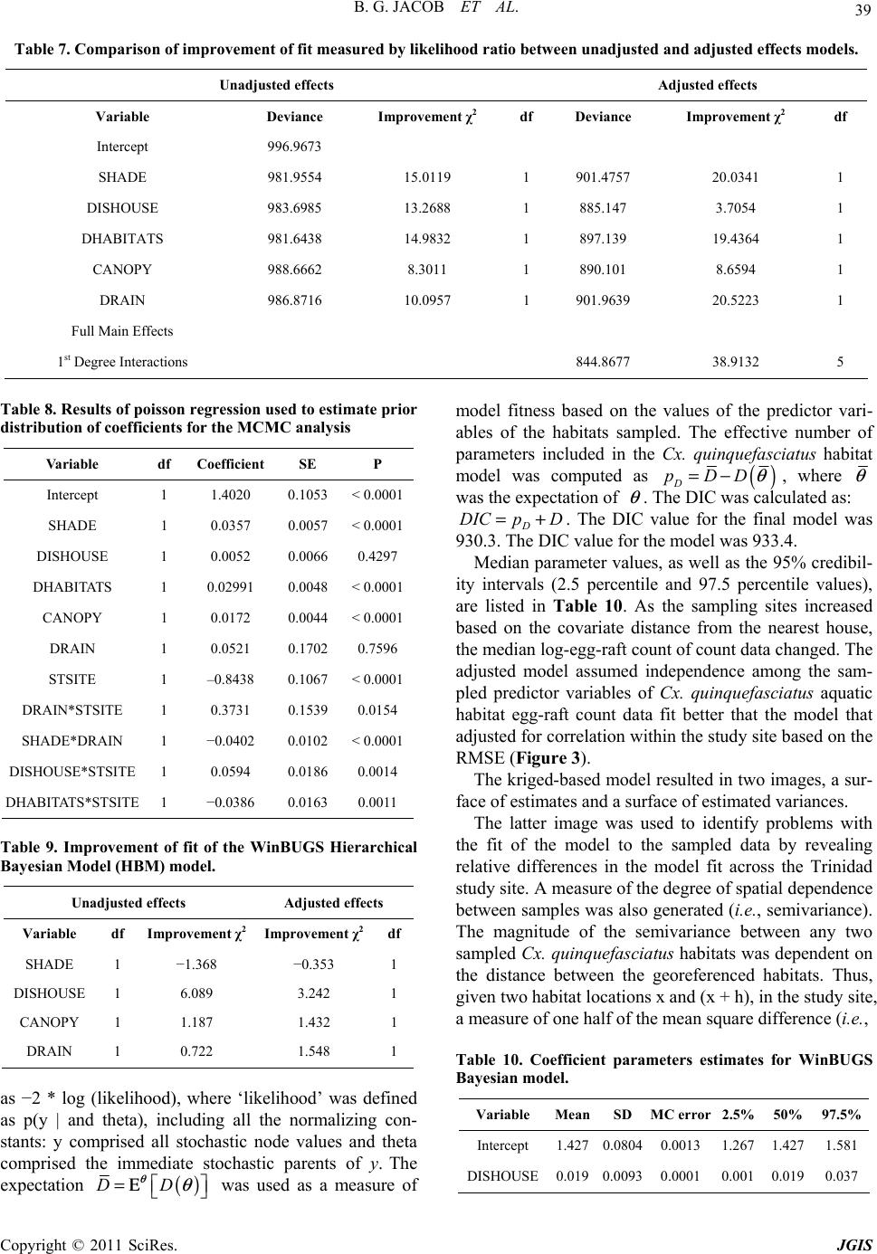

B. G. JACOB ET AL.
39
Table 7. Comparison of improvement of fit measured by likelihood ratio between unadjusted and adjusted effects models.
Unadjusted effects Adjusted effects
Variable Deviance Improvement χ2 df Deviance Improvement χ2 df
Intercept 996.9673
SHADE 981.9554 15.0119 1 901.4757 20.0341 1
DISHOUSE 983.6985 13.2688 1 885.147 3.7054 1
DHABITATS 981.6438 14.9832 1 897.139 19.4364 1
CANOPY 988.6662 8.3011 1 890.101 8.6594 1
DRAIN 986.8716 10.0957 1 901.9639 20.5223 1
Full Main Effects
1st Degree Interactions 844.8677 38.9132 5
Table 8. Results of poisson regression used to estimate prior
distribution of coefficients for the MCMC analysis
Variable df Coefficient SE P
Intercept 1 1.4020 0.1053 < 0.0001
SHADE 1 0.0357 0.0057 < 0.0001
DISHOUSE 1 0.0052 0.0066 0.4297
DHABITATS 1 0.02991 0.0048 < 0.0001
CANOPY 1 0.0172 0.0044 < 0.0001
DRAIN 1 0.0521 0.1702 0.7596
STSITE 1 –0.8438 0.1067 < 0.0001
DRAIN*STSITE 1 0.3731 0.1539 0.0154
SHADE*DRAIN 1 −0.0402 0.0102 < 0.0001
DISHOUSE*STSITE 1 0.0594 0.0186 0.0014
DHABITATS*STSITE 1 −0.0386 0.0163 0.0011
Table 9. Improvement of fit of the WinBUGS Hierarchical
Bayesian Model (HBM) model.
Unadjusted effects Adjusted effects
Variable df Improvement χ2 Improvement χ2df
SHADE 1 −1.368 −0.353 1
DISHOUSE 1 6.089 3.242 1
CANOPY 1 1.187 1.432 1
DRAIN 1 0.722 1.548 1
as −2 * log (likelihood), where ‘likelihood’ was defined
as p(y | and theta), including all the normalizing con-
stants: y comprised all stochastic node values and theta
comprised the immediate stochastic parents of y. The
expectation
()
DD
θ
θ =Ε 

was used as a measure of
model fitness based on the values of the predictor vari-
ables of the habitats sampled. The effective number of
parameters included in the Cx. quinquefasciatus habitat
model was computed as
()
D
pDD θ =− , where θ
was the expectation of θ . The DIC was calculated as:
D
DICpD=+. The DIC value for the final model was
930.3. The DIC value for the model was 933.4.
Median parameter values, as well as the 95% credibil-
ity intervals (2.5 percentile and 97.5 percentile values),
are listed in Table 10. As the sampling sites increased
based on the covariate distance from the nearest house,
the median log-egg-raft count of count data changed. The
adjusted model assumed independence among the sam-
pled predictor variables of Cx. quinquefasciatus aquatic
habitat egg-raft count data fit better that the model that
adjusted for correlation within the study site based on the
RMSE (Figure 3).
The kriged-based model resulted in two images, a sur-
face of estimates and a surface of estimated variances.
The latter image was used to identify problems with
the fit of the model to the sampled data by revealing
relative differences in the model fit across the Trinidad
study site. A measure of the degree of spatial dependence
between samples was also generated (i.e., semivariance).
The magnitude of the semivariance between any two
sampled Cx. quinquefasciatus habitats was dependent on
the distance between the georeferenced habitats. Thus,
given two habitat locations x and (x + h), in the study site,
a measure of one half of the mean square difference (i.e.,
Table 10. Coefficient parameters estimates for WinBUGS
Bayesian model.
Variable MeanSD MC error 2.5% 50%97.5%
Intercept 1.4270.08040.0013 1.267 1.427 1.581
DISHOUSE0.019 0.00930.0001 0.001 0.019 0.037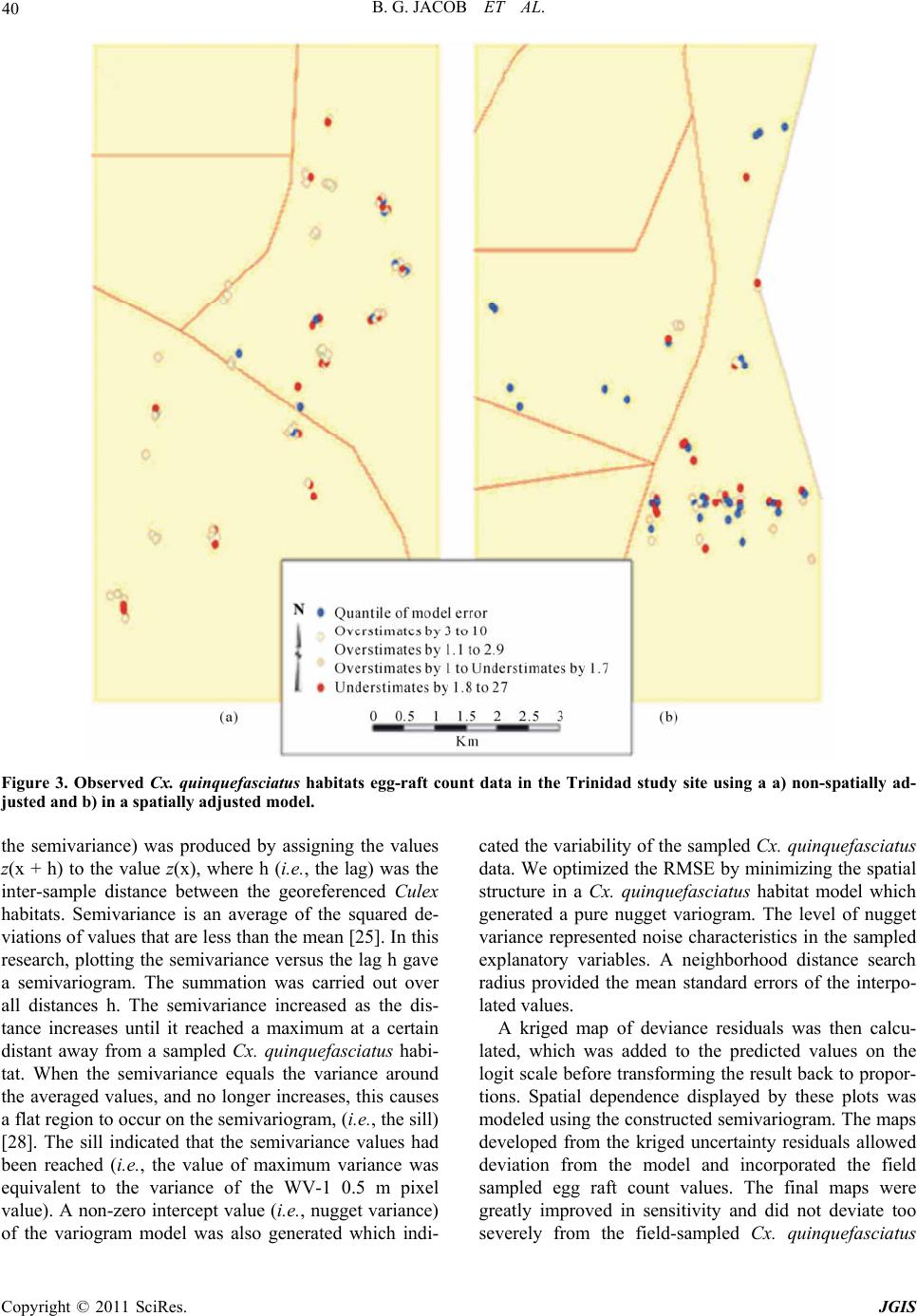

B. G. JACOB ET AL.
40
Figure 3. Observed Cx. quinquefasciatus habitats egg-raft count data in the Trinidad study site using a a) non-spatially ad-
justed and b) in a spatially adjusted model.
the semivariance) was produced by assigning the values
z(x + h) to the value z(x), where h (i.e., the lag) was the
inter-sample distance between the georeferenced Culex
habitats. Semivariance is an average of the squared de-
viations of values that are less than the mean [25]. In this
research, plotting the semivariance versus the lag h gave
a semivariogram. The summation was carried out over
all distances h. The semivariance increased as the dis-
tance increases until it reached a maximum at a certain
distant away from a sampled Cx. quinquefasciatus habi-
tat. When the semivariance equals the variance around
the averaged values, and no longer increases, this causes
a flat region to occur on the semivariogram, (i.e., the sill)
[28]. The sill indicated that the semivariance values had
been reached (i.e., the value of maximum variance was
equivalent to the variance of the WV-1 0.5 m pixel
value). A non-zero intercept value (i.e., nugget variance)
of the variogram model was also generated which indi-
cated the variability of the sampled Cx. quinquefasciatus
data. We optimized the RMSE by minimizing the spatial
structure in a Cx. quinquefasciatus habitat model which
generated a pure nugget variogram. The level of nugget
variance represented noise characteristics in the sampled
explanatory variables. A neighborhood distance search
radius provided the mean standard errors of the interpo-
lated values.
A kriged map of deviance residuals was then calcu-
lated, which was added to the predicted values on the
logit scale before transforming the result back to propor-
tions. Spatial dependence displayed by these plots was
modeled using the constructed semivariogram. The maps
developed from the kriged uncertainty residuals allowed
deviation from the model and incorporated the field
sampled egg raft count values. The final maps were
greatly improved in sensitivity and did not deviate too
severely from the field-sampled Cx. quinquefasciatus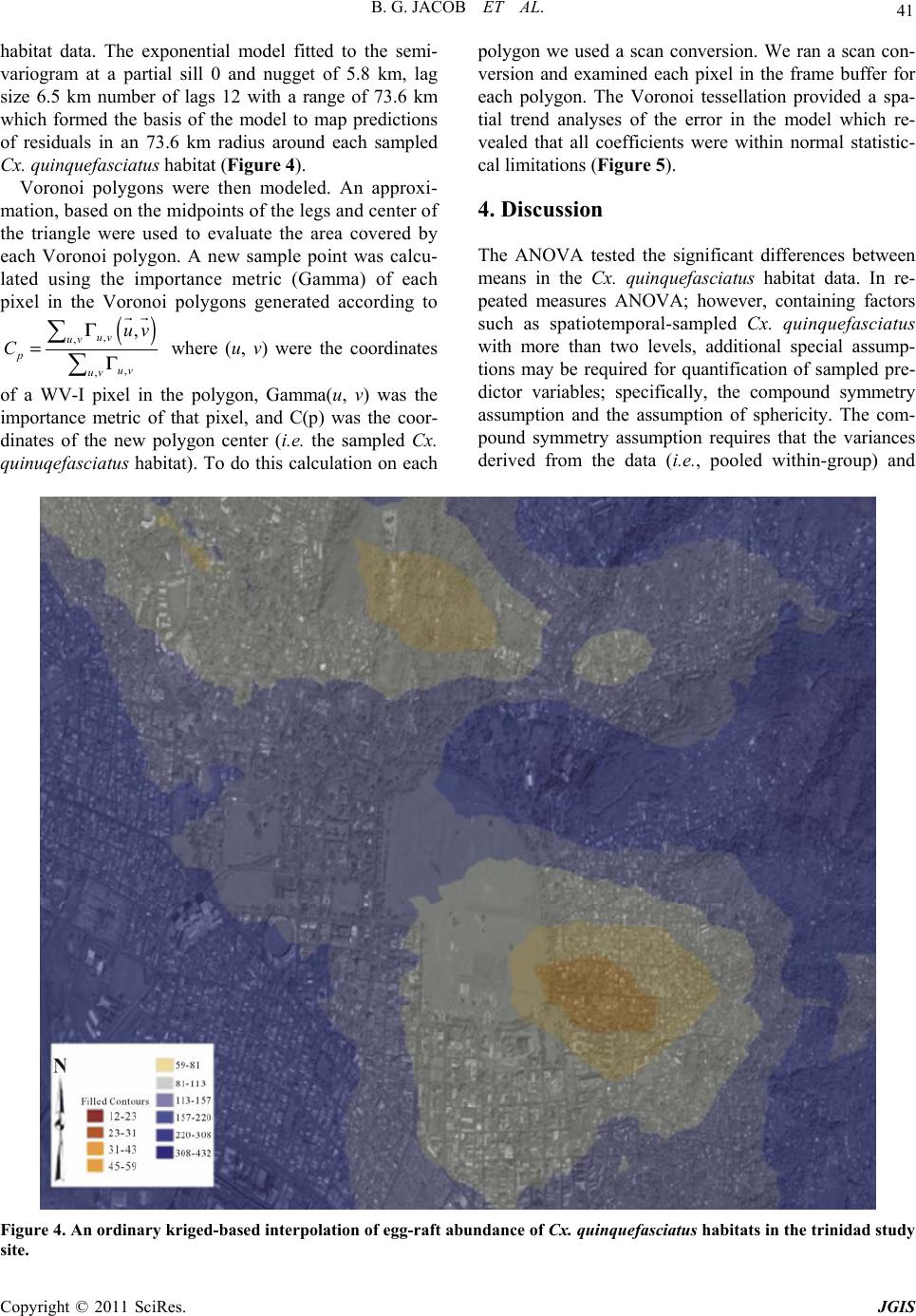

B. G. JACOB ET AL.
41
habitat data. The exponential model fitted to the semi-
variogram at a partial sill 0 and nugget of 5.8 km, lag
size 6.5 km number of lags 12 with a range of 73.6 km
which formed the basis of the model to map predictions
of residuals in an 73.6 km radius around each sampled
Cx. quinquefasciatus habitat (Figure 4).
Voronoi polygons were then modeled. An approxi-
mation, based on the midpoints of the legs and center of
the triangle were used to evaluate the area covered by
each Voronoi polygon. A new sample point was calcu-
lated using the importance metric (Gamma) of each
pixel in the Voronoi polygons generated according to
()
,
,
,
,
,
uv
uv
p
uv
uv
uv
C
Γ
=Γ



where (u, v) were the coordinates
of a WV-I pixel in the polygon, Gamma(u, v) was the
importance metric of that pixel, and C(p) was the coor-
dinates of the new polygon center (i.e. the sampled Cx.
quinuqefasciatus habitat). To do this calculation on each
polygon we used a scan conversion. We ran a scan con-
version and examined each pixel in the frame buffer for
each polygon. The Voronoi tessellation provided a spa-
tial trend analyses of the error in the model which re-
vealed that all coefficients were within normal statistic-
cal limitations (Figure 5).
4. Discussion
The ANOVA tested the significant differences between
means in the Cx. quinquefasciatus habitat data. In re-
peated measures ANOVA; however, containing factors
such as spatiotemporal-sampled Cx. quinquefasciatus
with more than two levels, additional special assump-
tions may be required for quantification of sampled pre-
dictor variables; specifically, the compound symmetry
assumption and the assumption of sphericity. The com-
pound symmetry assumption requires that the variances
derived from the data (i.e., pooled within-group) and
Figure 4. An ordinary kriged-based interpolation of egg-raft abundance of Cx. quinquefasciatus habitats in the trinidad study
site.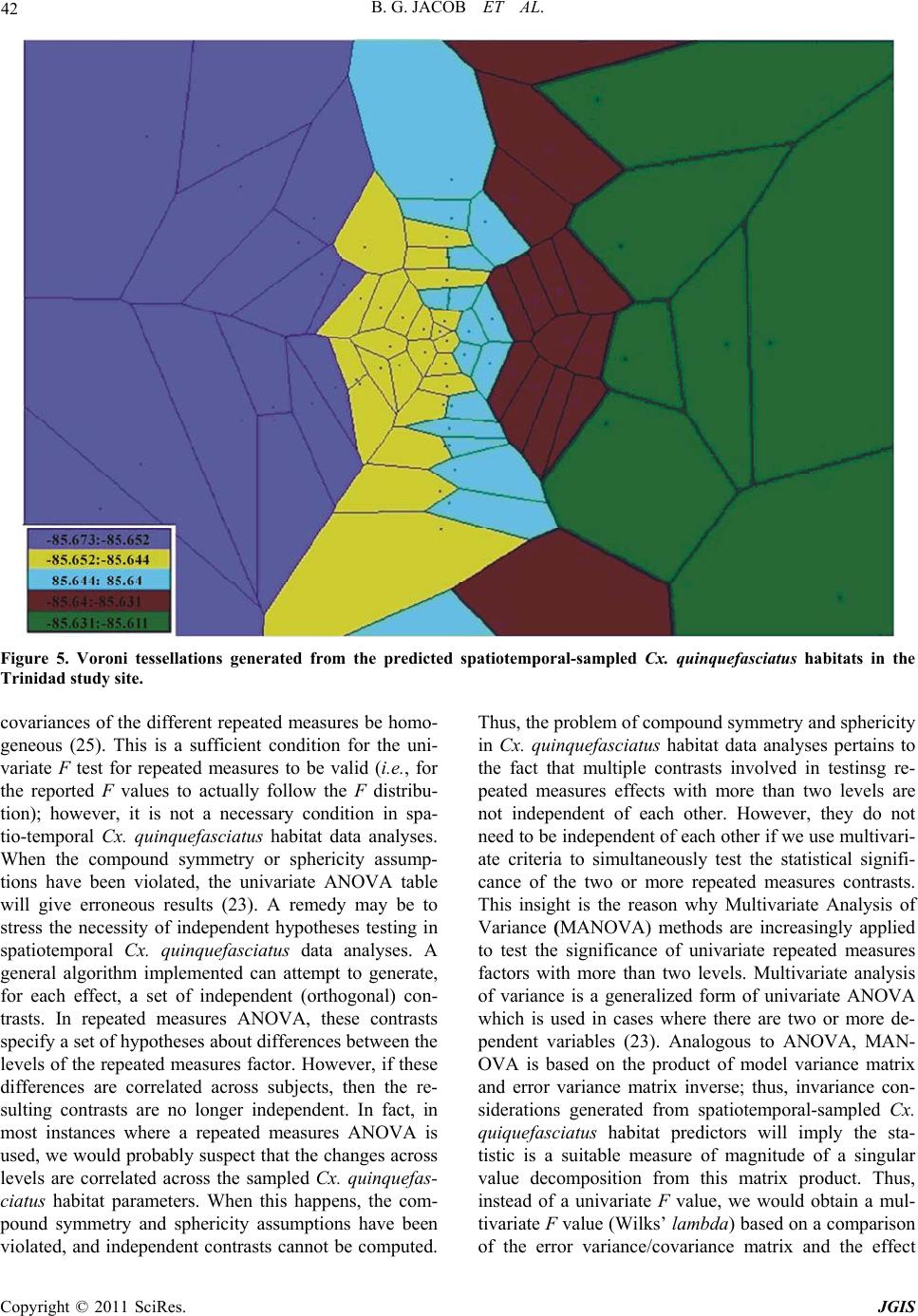

B. G. JACOB ET AL.
42
Figure 5. Voroni tessellations generated from the predicted spatiotemporal-sampled Cx. quinquefasciatus habitats in the
Trinidad study site.
covariances of the different repeated measures be homo-
geneous (25). This is a sufficient condition for the uni-
variate F test for repeated measures to be valid (i.e., for
the reported F values to actually follow the F distribu-
tion); however, it is not a necessary condition in spa-
tio-temporal Cx. quinquefasciatus habitat data analyses.
When the compound symmetry or sphericity assump-
tions have been violated, the univariate ANOVA table
will give erroneous results (23). A remedy may be to
stress the necessity of independent hypotheses testing in
spatiotemporal Cx. quinquefasciatus data analyses. A
general algorithm implemented can attempt to generate,
for each effect, a set of independent (orthogonal) con-
trasts. In repeated measures ANOVA, these contrasts
specify a set of hypotheses about differences between the
levels of the repeated measures factor. However, if these
differences are correlated across subjects, then the re-
sulting contrasts are no longer independent. In fact, in
most instances where a repeated measures ANOVA is
used, we would probably suspect that the changes across
levels are correlated across the sampled Cx. quinquefas-
ciatus habitat parameters. When this happens, the com-
pound symmetry and sphericity assumptions have been
violated, and independent contrasts cannot be computed.
Thus, the problem of compound symmetry and sphericity
in Cx. quinquefasciatus habitat data analyses pertains to
the fact that multiple contrasts involved in testinsg re-
peated measures effects with more than two levels are
not independent of each other. However, they do not
need to be independent of each other if we use multivari-
ate criteria to simultaneously test the statistical signifi-
cance of the two or more repeated measures contrasts.
This insight is the reason why Multivariate Analysis of
Variance (MANOVA) methods are increasingly applied
to test the significance of univariate repeated measures
factors with more than two levels. Multivariate analysis
of variance is a generalized form of univariate ANOVA
which is used in cases where there are two or more de-
pendent variables (23). Analogous to ANOVA, MAN-
OVA is based on the product of model variance matrix
and error variance matrix inverse; thus, invariance con-
siderations generated from spatiotemporal-sampled Cx.
quiquefasciatus habitat predictors will imply the sta-
tistic is a suitable measure of magnitude of a singular
value decomposition from this matrix product. Thus,
instead of a univariate F value, we would obtain a mul-
tivariate F value (Wilks’ lambda) based on a comparison
of the error variance/covariance matrix and the effect

B. G. JACOB ET AL.
43
variance/covariance matrix. The problem of compound
symmetry and sphericity pertains to the fact that multiple
contrasts involved in testing repeated measures of Cx.
quinquefasciatus habitat effects with more than two lev-
els are not independent of each other but, fortunately a
multivariate criteria can simultaneously test the statistical
significance of the two or more repeated measures con-
trasts. We thus endorse a MANOVA approach for spati-
otemporal data analyses of Cx. quinquefasciatus habitat
parameters as it simply bypasses the assumption of
compound symmetry and sphericity altogether.
The spatial hydrological model generated from the en-
vironmental-sampled Cx. quinquefasciatus covariates
revealed that elevation was an important variable in the
DEM model. Anderson et al. (2004) captured signify-
cantly more Culex quinquefasciatus in a variety of traps
(bird-baited, MMX mosquito magnet, CO2-baited CDC
trap) in the canopy (7.6 m) than at near ground level (1.5
m) [40]. In our research local differences among WV-1
DEM grid cells were also analyzed to calculate slope and
other land surface parameters using relative and absolute
accuracy estimates for determining the statistical signifi-
cance of terrain-related parameters associated to the Cx.
quinquefasciatus habitats. In this research the slope gra-
dient was defined as the maximum rate of change in alti-
tude (i.e., tan (Θ), aspect (ψ) as the compass direction of
this maximum rate of change). Slope is defined by a
plane tangent to a topographic surface, as modeled by the
DEM at a point, whereby, it is classified as a vector; as
such it has a quantity (gradient) and a direction (aspect).
More analytically, the slope gradient at a sampled Cx.
quinquefasciatus habitat in the Trinidad study site was
the first derivative of elevation (Z) with respect of the
slope (S), where S was in the aspect direction (ψ). We
calculated the first derivative of a function at a sampled
habitat as the angular coefficient of the tangent to the
function of a sampled habitat. The resolution of our
WV-1 DEM quantified the georeferenced explanatory
covariates at each 0.5m pixel (i.e., absolute accuracy). At
the same time the relative accuracy of the sampled data
generated a geometrically correct reference frame for
validating the covariate elevation associated with the
sampled Cx. quinquefasciatus habitats. WV-1 DEMs can
allow for hydrologic modeling, view-shed determination,
slope/aspect analyses, and 3-d surface visualization of
georeferenced terrain-related parameters associated to
spatiotemporal-sampled Cx. quinquefasciatus habitat
data.
In the regression model, PROC MIXED quantified
correlations among error measurements using random
effects estimates and random regression coefficients.
PROC MIXED used three options for the method of es-
imation including: 1) Maximum Likelihood (ML); 2)
Restricted or Residual maximum likelihood (REML),
which was the default method; and, 3) Minimum Vari-
ance Quadratic Unbiased Estimation (MIVQUE). In this
research, the ML was the regular maximum likelihood
method as the Cx. quinquefasciatus parameter estimates
maximized the likelihood function, while the REML was
a variant of maximum likelihood. The sample mean was
the maximum likelihood estimator of the sampled habitat
population mean, based on the egg-raft count data. The
sample variance was also a close approximation to the
maximum likelihood estimator of the immature sampled
variance. REML estimated the variance parameters using
a marginal likelihood which produced unbiased estimates.
REML estimators generated estimates from the spatio-
temporal-sampled parameters by maximizing only that
part of the likelihood function that was invariant to the
fixed effects part of the linear model. The variance of a
quadratic function of the random variables in the linear
model was then minimized to obtain locally best unbi-
ased estimators of the variance components. The matri-
ces of these quadratics were computed from relationship
matrices and from prior estimates of variances used in
the model equations.
In the Bayesian matrix we were able to instantiate the
nodes directly which was equivalent to supplying, a
measurement for a radius based on the distribution of the
georeferenced Cx. quinquefasciatus habitats. We were
able to quantify an uncertainty estimate in our likelihood
information by supplying a probability distribution over
a set of radii generated from the sampled data. We used a
backward propagation to compute the node probabilities.
The error gradients were then propagated in any direc-
tion throughout the Bayesian framework. This type of
probability propagation allowed choosing between the
sampled predictor variables using the computed prob-
ability of each sampled covariate value based on one or
more of the nodes.
Our Bayesian approach allowed flexible model fitting
and estimation and geomapping of all “high risk” Cx.
quinquefasciatus habitats based on sampled egg-raft
count data in the study site. The MCMC algorithm for
the Cx. quinquefasciatus egg-raft count model produced
a sequence of parameter vectors that represented random
draws from the posterior distribution. The DIC com-
prised two goodness-of-fit measures and the posterior
distribution of the deviance, which was the number of
effective sampled habitat covariates for measuring com-
plexity in our Cx. quinquefasciatus model. Habitats with
high egg-raft counts were compared with the results of a
Monte Carlo simulation, which established the probabili-
ties and occurrences of these habitats. Our results indi-
cated that likelihood weights influenced the resulting
posterior distributions of the field and remote-sampled

B. G. JACOB ET AL.
44
Cx. quinquefasciatus egg-raft count parameters, which,
in turn influenced the spatial trends in the variance un-
certainty estimates for model prediction. Distance from
the nearest house was a significant predictor associated
with prolific habitats in the Trinidad study site.
Environmental factors commonly associated with Cx.
quinquefasciatus habitats include the distance from the
nearest human habitation. The location of WNV cases at
the place of residence can be based on the fact that Culex
mosquitoes are crepuscular feeders, and are most likely
to come in contact with people while they are at home
during the evening hours. Because egg-laying is a spatial
process dependent upon the location of the focal habitat
relative to sources of gravid mosquitoes, habitats closer
to human inhabitations tend to receive more eggs and
thus are more productive if conspecific competition is
negligible [29]. Furthermore, housing age can also play a
big role in the explanation of the focal areas. This is ex-
pected since older houses have poorer drainage systems
and open foundations which may provide larval and
adult habitats. For example, houses built in the post
World War II era in the study site may suffer from a
general inattention. These houses may contain catch ba-
sins, rich with organic material which are breeding
grounds for Culex mosquitoes. Most of the Culex species
require organic-rich water for larval development and are
commonly found in high numbers in artificial containers,
unattended pools, retention ponds, storm drains, catch
basins, sewage systems and treatment plants [41,42].
Furthermore, combined sewage and street runoff dis-
charges into natural waterways are considered the main
sources of urban stream pollution, which are associated
to WNV as Culex mosquitoes proliferate in eutrophic
hydrological networks. The identification of social fac-
tors that characterize these focal areas in the Trinidad
study site may also provide insight into human risk and
can help to target control and prevention strategies. Fu-
ture analyses should explicitly test whether enzootic and
bridge transmission are related to human population fac-
tors includeing household income, population age, age of
housing, housing density, and population density. Since
it can be assumed from this analysis that the WNV is
transmitted near a person’s residence in the Trinidad
study site, extensive engineering to improve the runoff of
water in residential areas should be considered.
A framework for assessing autocorrelation in residual
error from the spatial analyses was constructed in SAS/
GIS®. We generated a semiparametric filtering model
using proxy variables constructed from the spatiotempo-
ral-sampled georeferenced explanatory variables. In our
Cx. quinquefasciatus habitat model, the misspecification
terms was replaced by the proxy vari- ables for imple-
menting a conditional covariance matrix employing the
autoregressive specification. An unknown misspecifica-
tion term can be approximated by a set of spatial proxy
variables [38]. After modeling the mis- specification
terms, the remaining residuals ˆ
ε become white noise.
This result implied that the estimated re- gression pa-
rameters ˆ
β
were unbiased for the basic regression
model, *
yX
β
ε =+
, where * ε incorpo- rated the
misspecification term and the white-noise dis- turbances.
This allowed us to calibrate the autoregressive models.
All of these eigenvectors exhibited weak posi- tively
autocorrelated spatial patterns in the habitat pa- rameter
estimates. Local weather patterns, mosquito con- trol
programs and movement of hosts can have spatial ex-
pressions, which cause immature Culex mosquetoes to
aggregate in geographic space rendering positive auto-
correlation in sampled predictor variables [8,26].
In this research, we used an Ordinary interpolation in
ArcGIS® for identifying initial spatial structures in the
sampled Cx. quinquefasciatus habitats and for quantify-
ing the variance and autocorrelation in the data. The es-
timation method determined the best linear unbiased es-
timator. It was linear since the estimated values were
weighted linear combinations of the spatiotemporal-
sampled data and it was unbiased because the mean of
the error was zero. For determining the optimal predict-
tors, a semivariogram was constructed which expressed
the spatial variation in the sampled data. In this research
the variogram [i.e., 2γ(x,y)] was a function describing the
degree of spatial dependence between the sampled Cx.
quinquefasciatus habitats [i.e., Z(x)]. This was defined as
the expected squared increment of the values between
the sampled habitat locations x and y. Our semivariogram
was nonnegative since it was the expectation of a square.
The covariance function was related to variogram by
2γ(x,y) = C(x,x) + C(y,y) - 2C(x,y). In this research, the
γ(x,y) = E(|Z(x) − Z(y)|2) = γ(y,x) was a symmetric func-
tion, consequently, γs(h) = γs(- h) was an even function.
A function is a semivariogram if, and only if, it is a con-
ditionally negative definite function, i.e. for all weights
1,,
N
ww subject to 10
N
i
iw ==
 and locations
1,,
N
x
x, thus, it holds:
()
11 ,0
NN
iijj
ij
wxxw γ
== ≤
 [28]. The function corre-
sponded to the fact that the variance [i.e., va r(X) of
()
1
N
ii
j
X
wZ x
=
= generated from the sampled Cx.
quinquefasciatus data was given by the negative of this
double sum, which in this research was nonnegative. All
spatial dependence was quantified in the model. If a sta-
tionary random field has no spatial dependence (i.e. C(h)
= 0 if 0h≠ the semivariogram is the constant var(Z(x))
everywhere except at the origin, where it is zero [28].
Theoretically, at zero separation distance (lag = 0), the
semivariogram value is zero in a predictive vector mos-

B. G. JACOB ET AL.
45
quito habitat distribution model; however, at an infini-
tesimally small sampled habitat distances, the semi-
variogram often exhibits a nugget effect (i.e., measure-
ment errors or spatial sources of variation at distances
smaller than the sampling interval), which is some value
greater than zero [16]. Additionally, since the random field
was stationary and ergodic, the
()() ()
var
lim s
h
hZx
γ
→∞ =
corresponded to the variance generated by the Cx. quin-
que fa sc i atu s habitat data. We defined a practical range
and defined the distance at which 95% of the sill was
reached for the asymptotic variogram model. The semi-
variogram calculated estimates of the surface at the dif-
ferent habitat locations. The increase in the semivario-
gram values with increasing lags diminished with dis-
tance and leveled off, at around 70 km (i.e., the range or
active lag distance). This was the approximate distance at
which spatial autocorrelation between the Cx. Quinque-
fasciatus habitat data point pairs ceased or became much
more variable. In the future sampling variograms should
be constructed using spatiotemporal-sampled Cx. Quin-
que fa sc i atu s habitat data. The sampling variogram,
unlike the semivariogram, shows where a significant
degree of spatial dependence in the sample space or
sampling unit dissipates into randomness when the vari-
ance terms of a temporally or in-situ ordered set are
plotted against the variance of the set and the lower lim-
its of its 99% and 95% confidence ranges [28]. Sam-
pling variograms may quantify extraneous measurement
variances before spatial dependence is verified in a pre-
dictive Cx. quinquefasciatus habitat distribution model.
In this research interpolation accuracy was also
measured by the natural logarithm of the mean squared
interpolation error and Voroni polygons which revealed
all uncertainty effects while quantifying several covariate
interaction terms in Euclidean space. The Voroni cells
generated were a d-dimensional polytope (i.e., a convex
hull of a finite set of georeferenced points). A set of
hyperplanes were generated using the polygonal shapes
around each sampled Cx. quinuqefasciatus habitat in the
Trinidad study site. If S contains only two points, a and b,
then the set of all points equidistant from a and b is a
hyperplane-an affine subspace of codimension 1 [28]. The
set of the polytopes covered the whole space and was the
Voronoi tessellation corresponding to the georeferenced
Cx. quinquefasciatus habitats. The convex Voronoi
polygons were visualized as space-filling polygons
constructed around the dataset of the sampled covariates
(i.e.,Voronoi centers), such that each polygon contained
all points closer to its Voronoi center than to the center of
any other polygon. The relationship of the Voronoi
centers to edges of polygons were used to test whether any
convex tessellation existed in the polygons. This test
amounted to finding Voronoi centers that best fit the given
tessellation. In this research, Voronoi centers were found
by solving two systems of linear equations. These
equations represented 1) conditions on the slope of
polygon edges relative to the slope of lines through
Voronoi centers, and 2) conditions on the distance from
edges to Voronoi centers. Least squares and constrained
least-squares solutions were used to solve the two systems.
In order to quantitatively characterize the error in the
interpolation model, we examined normalized cell size
distribution related to the homogenous and inhomogeneous
fixation densities (i.e., Cx. quinquefasciatus habitat
egg-raft count), which provided additional insight as to
how the convex tessellations varied between the Voronoi
polygons. A goodness-of-fit statistic was derived using the
Voronoi tessellations which determined the error propa-
gation in the multivariate model. The Voroni residuals
reflected sampling errors and analytical errors based on the
sampled Cx. quinquefasciatus habitat egg-raft count
density.
In the future new network nodes using Dirichlet
tessellations in spatiotemporal-sampled Cx. quinque-
fasciatus habitats should be analyzed. For example,
Okabe and Satoh, (2008) have developed a software
package, SANET, which can be installed as an ArcGIS
add-in for “Spatial Analysis on a Network” for
determining new network nodes [43]. The SANET
software includes a network-based Voronoi tool, very
similar to some of the network analysis tools provided in
ArcGIS itself and in network-oriented packages such as
TransCAD and Cube. The point set (i.e., off-network sites)
can be linked to the nearest network edge, and then
non-directed network Voronoi regions can be generated
from georferenced Cx. quinquefasciatus habitat locations
using shortest path distances. Separate inward and
outward-directed Voronoi regions can then be computed
and each habitat can be derived using unweighted
calculations.
For future research, the risk of WNV transmission in
the Trinidad study site should also be investigated using
wild bird roosting behavior and seasonal migratory pat-
tern data. Quantifying WNV amplification at a local
scale, with explicit attention to distances measurements
from mosquito and hatch-year bird sites and human
habitation areas may affect timing of infection in birds,
mosquitoes, and humans. Seropositive resident and mi-
gratory birds have been documented along the Atlantic
and Mississippi flyways into the Caribbean [2]. While
transient birds may suggest a means by which WNV has
rapidly spread across North and Central America, resi-
dent breeding birds may be more critical for zoonotic
transmission in Trinidad [44-47]. In North America, high
seroprevalence is associated with avian species that
breed year-round and live close to humans (e.g. Ameri-
can robin, House sparrow, Mourning dove, Northern

B. G. JACOB ET AL.
46
cardinal, Northern mockingbird), though other wild birds
may be important [47-49]. In contrast to the urban avian
species commonly associated as WNV hosts in North
America, avian WNV hosts that occur in Trinidad are
often non-urban, wild bird species [2]. Caribbean birds
that have tested seropositive for WNV and are resident to
Trinidad or breed seasonally in Trinidad include: Ba-
nanaquits (Coereba flaveola), Palm-tanagers (Phaenico-
philus palmarum), and Grossquit species [2]. Since the
significance of avian species in WNV transmission may
relate to their host competency, natural exposure to
mosquito vectors and spatiotemporal availability, an
avian GIS-based model using spatial filter eigenvectors
and Bayesian estimates might be able to generate glob-
ally asymptotically stable parameters while quantifying
the amplification cycle prior to bridge vector involve-
ment. Bridge vectors are mosquito species that readily
feed on humans and mammals [2].
In conclusion, correlation estimates generated from the
WV-1 DEM revealed that the terrain covariate elevation
was significantly associated with the Cx. quinquefasciatus
habitats sampling sites. The spatial hydrological model
allowed for hydrologic modeling, view-shed deter-
mination, slope/aspect analyses, and 3-d surface visua-
lization of the georeferenced parameters associated to Cx.
quinquefasciatus habitat data. Elevation data was
represented in the WV-1 DEM by including gridded data
where the terrain covariate was estimated for each cell in a
regular grid, a triangular irregular network, and contours.
The coefficients from the decomposition of the sampled
predictor variables were then entered into a Bayesian
matrix. This framework allowed flexible model fitting,
estimation, and mapping of all high risk habitats based on
field-sampled egg-raft count data using a MCMC
specification. Residual estimates were then analyzed with
an eigenvector spatial filtering algorithm which trans-
formed all the georferenced predictor variables containing
spatial dependence into covariates free of spatial
dependence by partitioning the original sampled habitat
data and the sampled egg-raft abundance count data into
two synthetic variates: 1) a spatial filter variate capturing
latent spatial dependency and 2) a non-spatial variate that
was free of spatial dependence. The geographic distribution
of the sampled habitats based on the egg-raft counts
exhibited positive autocorrelation in all models tested:
log-egg-raft counts aggregated in geo-space. The procedure
accounted for 17 % pseudo-replicated information in the
datasets. All models were then adjusted based on the
residual estimates form the eigenfunction decomposition
algorithm and then kriged. The sill indicated that the
semivariance values had been reached (i.e., the value of
maximum variance was equivalent to the variance of a
0.5m pixel value), while a non-zero intercept value (i.e.,
nugget variance) of the varigram model was indicative of
the variability of the field and remotesampled Cx.
quinquefasciatus data. A simple quantitative measure of
the interpolation performed was determined by generating
RMSE values for the models and by constructing Voroni
polygons. Optimizing the RMSE by minimizing the
spatial structure in a Cx. quinquefasciatus habitat model
generated a pure nugget variogram, of which the level of
nugget variance represented noise characteristics in the
predictor variables. Interpolation accuracy tests measured
by the natural logarithm of the mean squared interpolation
error and the Voroni polygons revealed all error effects of
the parameter estimates in the kriged-based model and
quantified the covariate interaction terms. Newer GIS
software, WV-I data and spatial statistics can implement
larval control strategies by targeting prolific habitats of
Cx. quinquefasciatus based on field-sampled count data in
Trinidad.
In the future high quality spatial autoregressive and
surface models should be constructed using spatiotem-
poral-sampled Cx. quinquefasciatus and other mosquito
habitat data and Worldview-2 (WV-2) imagery for im-
proving sensitivity in LULC, elevation and kriged-based
interpolation parameters in Trinidad. On October 8, 2009
Digitalglobe launched WV-2 which is the first high
resolution commercial satellite to offer 8-band capability
with high accuracy, agility and spectral diversity (www.
digitalglobe.com). This allows the creation of accurate
Cx. quinuqefasciatus habitat maps without the need of
GCPs. A wide range of features can be extracted using
the traditional four spectral bands but WV-2 offers the
addition of the Coastal Yellow, Red edge and shorter
wave NIR bands which may provide a wider range of
potential derivatives for targeting prolific Cx. Quinque-
fasciatus and other mosquito habitats. For example, the
Coastal-blue bands can be used for bathymetry, benthic,
wetland and atmospheric modeling which can assist in
detecting subtle differences in land cover and coastal
features associated with prolific mosquito habitats.
Probably the best feature of WV-2 for geomapping Cx.
quinquefasciatus and other mosquito habitats, however,
is the ability to derive algorithms and functions from new
band combinations for feature extraction and improved
classification. For example, the Red-edge NIR band can
identify plant health and age through chlorophyll produc-
tion while the yellow band in conjunction with the Red
Edge band can provide agricultural applications and iron
oxide mineralogy which can model moisture content. Thus,
WV-2 can provide detailed imagery for precise map gen-
eration, LULC change detection, construction of DEMs
and autoregressive predictive models. WV-2 data can
further help implement a remote-based habitat surveil-
lance in Trinidad and in other regions.

B. G. JACOB ET AL.
47
5. Acknowledgements
We acknowledge the data collection provided by the
Ministry of Health in Trinidad and Tobago and the De-
partment of Life Sciences, University of the West Indies,
St. Augustine, and Trinidad. This research was funded by
the National Institute of Health Grant U01A154889
(Novak Robert) University of Alabama at Birmingham
and from the Government of Trinidad and Tobago,
GTTGF-6 (Chadee Dave).
6. References
[1] D. Nash, F. Mostashari, A. Fine, J. Miller, D. O’Leary, K.
Murray, A. Huang, A. Rosenberg, A. Greenberg, M.
Sherman, S. Wong, G. L. Campbell, J. T. Roehrig, D. J.
Gubler, W. J. Shieh, S. Zaki, P. Smith and M. Layton,
“The Outbreak of West Nile Virus Infection in the New
York City Area in 1999,” The New England Journal of
Medicine, Vol. 344, 2001, pp. 1807-1814.
doi:10.1056/NEJM200106143442401
[2] N. Komar and G. C. Clark, “West Nile Virus Activity in
Latin America and the Caribbean,” Revista Panameri-
cana de Salud Pública, Vol. 19, 2006, pp. 112-117.
doi:10.1590/S1020-49892006000200006
[3] M. J. Turell, M. R. Sardelis, M. L. O’Guinn and D. J.
Dohm, “Potential Vectors of West Nile Virus in North
America. Curr,” Top Microbiol. Immunol, Vol. 267, 2002,
pp. 241-252.
[4] B. G. Jacob, R. L. Lampman, M. P. Ward, E. J. Muturi, J.
A. Morris, E. X. Caamano and R. J. Novak, “Geospatial
Variability in the Egg Raft Distribution and Abundance
of Culex Pipiens and Culex Restuans in Urbana-Cham-
paign, Illinois,” International Journal of Remote Sensing,
Vol. 30, 2009, pp. 2005-2019.
doi:10.1080/01431160802549195
[5] B. G. Jacob, W. Gu, E. J. Muturi, E. X. Caamano, J. M.
Morris, R. Lampman, R. J. Novak, “Developing Opera-
tional Algorithms Using Linear and Non-Linear Least
Squares Estimation in Python® for Identification of Culex
Pipiens and Culex Restuans Aquatic Habitats in a Mos-
quito Abatement District (Cook County, Illinois),” Geo-
spat Health, Vol. 3, 2009, pp. 23-31.
[6] J. K. Meece, J. S. Henkel, L. Glaser, K. D. Reed, “Mos-
quito Surveillance for West Nile Virus in Southeastern
Wisconsin-2002,” Clinical Medicine & Research Vol. 1,
2003, pp. 37-42. doi:10.3121/cmr.1.1.37
[7] F. W. Kutz, T. G. Wade and B. B. Pagac, “A Geospatial
Study of the Potential of Two Exotic Species of Mosqui-
toes to Impact the Epidemiology of West Nile Virus in
Maryland,” Journal of the American Mosquito Control
Association, Vol. 19, 2003, pp. 190-198.
[8] D. A. Griffith, “A Comparison of Six Analytical Disease
Mapping Techniques as Applied to West Nile Virus in
the Coterminous United States,” International Journal of
Health Geographics, Vol. 4, 2005, pp. 18-26.
doi:10.1186/1476-072X-4-18
[9] U. Kitron, “Risk Maps: Transmission and Burden of
Vector-Borne Diseases,” Parasitol Today, Vol. 16, 2000,
pp. 324-325. doi:10.1016/S0169-4758(00)01708-7
[10] D. J. Rogers and S. E. Randolph, “Studying the Global
Dis- tribution of Infectious Diseases Using GIS and RS,”
Na- - ture Reviews Microbiology, Vol. 1, 2003, pp.
231-237.
[11] S. I. Hay, J. A. Omumbo, M. H. Craig and R. W. Snow,
“Earth Observation, Geographic Information Systems and
Plasmodium Falciparum Malaria in Sub-Saharan Africa,”
Advances in Parasitol,Vol. 47, 2000.
[12] E. P. Pegoraro, M. J. Monson, R. K. Rey, A. Barron-Gaf-
ford and C. B. Osmond, “The Effect of Elevated CO2,
Soil and Atmospheric Water Deficit and Seasonal
Phenology on Leaf and Ecosystem Isoprene Emission,”
Functional Plant Biology, Vol. 34, 2007, p. 774.
doi:10.1071/FP07021
[13] J. S. Brownstein, T. R. Holfold, D. Fish, “Enhancing
West Nile Virus Surveillance, United States,” Emerging
Infectious Diseases, Vol. 10, 2004, pp. 1129-1133.
[14] N. Komar, S. Langevin, S. Hinten, N. Nemeth, E. Ed-
wards, D. Hettler, B. Davis, R. Bowen, M. Bunning,
“Experimental Infection of North American Birds with
the New York 1999 Strain of West Nile Virus,” Emerg-
ing Infectious Diseases, Vol. 9, 2003, pp. 311-322.
[15] L. R. Petersen, A. A. Marfin, D. J. Gubler, “West Nile
Virus,” JAMA, the Journal of the American Medical As-
sociation, Vol. 4, No. 290, 2003, pp. 524-528.
[16] B. G. Jacob, N. D. Burkett-Cadena, J. C. Luvall, S. H.
Parcak, C. J. W. McClure, L. K. Estep, G. E. Hill, E. W.
Cupp and R. J. Novak, “Developing GIS-Based Eastern
Equine Encephalitis Vector-Host Models in Tuskegee, Ala-
Bama,” International Journal of Health Geographics, Vol.
9, 2010, p. 12. doi:10.1186/1476-072X-9-12
[17] E. Mushinzimana, S. Munga, N. Minakawa, L. Li, C. C.
Feng, L. Bian, U. Kitron, C. Schmidt, L. Beck, G. Zhou
and A. K. Githeko, “Landscape Determinants and Re-
mote Sensing of Anopheline Mosquito Larval Habitats in
the Western Kenya Highlands,” Malaria Journal, Vol. 5,
2006, p. 13. doi:10.1186/1475-2875-5-13
[18] J. Shaman, J. F. Day and M. Stieglitz, “Drought-Induced
Amplification and Epidemic Transmission of West Nile
Virus in Southern Florida,” Journal of Medical Entomol-
ogy, Vol. 42, No. 2, 2005, pp. 134-141.
doi:10.1603/0022-2585(2005)042[0134:DAAETO]2.0.C
O;2
[19] J. R. Jensen, “Remote Sensing of Urban Suburban Infra-
structure and Socio-Economic Attributes,” Photogram-
metric Engineering and Remote Sensing, Vol. 5, No. 65,
2005, pp. 611-622.
[20] B. G. Jacob, E. J Muturi, E. X. Caamano, J. T. Gunter, E.
Mpanga, R. Ayine, J. Okelloonen, J. P. M. Nyeko, J. I.
Shililu, J. I. Githure, J. L. Regens and R. J. Novak, “Hy-
dro- logical Modeling of Geophysical Parameters of Ar-
boviral and Protozoan Disease Vectors in Internally Dis-
placed People Camps in Gulu, Uganda,” International
Journal of Health Geographics, Vol. 7, 2008, pp. 1-11.
doi:10.1186/1476-072X-7-11

B. G. JACOB ET AL.
48
[21] B. G. Jacob, D. A. Griffith and R. J. Novak, “Decompos-
ing Malaria Mosquito Aquatic Habitat Data into Spatial
Autocorrelation Eigenvectors in a SAS/GIS® Module,”
Transactions in GIS Vol. 12, 2008, pp. 341-364.
doi:10.1111/j.1467-9671.2008.01104.x
[22] C. N. Theophilides, S. C. Ahearn, E. S. Binkowski, W. S.
Paul and K. Gibbs, “First Evidence of West Nile Virus
Am- plification and Relationship to Human Infections,”
Inter- national Journal of Geographical Information
Science, Vol. 20, 2006, pp. 103-115.
doi:10.1080/13658810500286968
[23] T. G. Andreadis, J. F. Anderson and C. R. Vossbrink,
“Mos- quito Surveillance for West Nile Virus in Con-
necticut, 2000: Isolation from Culex Pipiens, Cx. Restu-
ans, Cx. Salinarius, and Culiseta Melanura,” Emerging
Infectious Diseases, Vol. 7, 2001, pp. 670-674.
doi:10.3201/eid0704.010413
[24] M. Eidson, J. Miller, L. Kramer, B. Cherry and Y. Hagi-
wara, “Dead Crow Densities and Human Cases of West
Nile Virus New York State 2000,” Emerging Infectious
Dis- eases, Vol. 7, 2001, pp. 662-664.
doi:10.3201/eid0704.010411
[25] M. Kulldroff, “A Spatial Scan Statistic,” Community
Statistical Theory Methods, Vol. 26, 1997, pp. 1481-1496.
doi:10.1080/03610929708831995
[26] B. G. Jacob, E. Muturi, J. Mwangangi, J. Funes, J. Shililu,
J. Githure and R. J. Novak, “Remote and Field Level
Quantification of Vegetation Covariates for Malaria
Mapping in Three Rice Agro-Village Complexes in Cen-
tral Kenya,” International Journal of Health Geographics,
Vol. 6, 2007, pp. 21-28. doi:10.1186/1476-072X-6-21
[27] I. Kleinschmidt, M. Bagayoko, G. P. Y. Clarke, M. Craig
and D. L. Le Sueur, “A Spatial Statistical Approach to
Ma- laria Mapping,” International Epidemiology Asso-
ciation, Vol. 29, No. 2, 2000, pp. 355-361.
[28] N. Cressie, “Aggregation in Geostatistical Problems,”
Geostatistics troia, 1992.
[29] W. Gu and R. J. Novak, “Habitat-Based Modeling of
Impacts of Mosquito Larval Interventions on Entomo-
logical Inoculation Rates, Incidence, and Prevalence of
Malaria,” American Journal of Tropical Medicine and
Hygiene, Vol. 73, 2005, pp. 546-552.
[30] B. G. Jacob, D. A. Griffith, E. J. Muturi, E. X. Caamano,
J. I. Githure, J. T. Gunter, R. J. Novak, “A Heteroskedas-
tic Error Covariance Matrix Estimator Using a
First-Order Conditional Autoregressive Markov Simula-
tion for Deriving Asymptotical Efficient Estimates from
Ecological Sampled Anopheles Arabiensis Aquatic Habi-
tat Covariates,” Malaria Journal, Vol. 8, 2009, pp.
216-224. doi:10.1186/1475-2875-8-216
[31] D. Chadee, “Key Premises, a Guide to Aedes Aegypti
(Diptera: Culicidae) Surveillance and Control,” Bulletin
of Entomological Research, Vol. 94, 2004, pp. 201-207.
doi:10.1079/BER2004297
[32] J. P. Bradbury, B. Leyden, M. Salgado-Labouriau, Lewis,
W. M. Jr., C. Schubert, M. W. Binford, D. G. Frey, D. R.
Whitehead and F. W. Weibezahn, “Late Quaternary Envi-
ronmental History of Lake Valencia,” Ven. Science, Vol.
4, 1981, pp. 18-26.
[33] J. R. Flenley, “The Equatorial Rain Forest: A Geological
History,” Butterworth, London, Vol. 9, 1979, p. 162.
[34] J. S. Beard, “The Mora Forests of Auburn, British West
Indies,” Journal of Ecology, Vol. 33, 1946, pp. 173-192.
doi:10.2307/2256464
[35] D. D. Chadee, “Indoor and Outdoor Host-Seeking
Rhythms of Anopheles Albitarsis (Diptera: Culicidae) in
Trinidad, West Indies,” Journal of Medical Entomology,
Vol. 29, 1992, pp. 567-569.
[36] B. G. Jacob, P. G. Nelson, R. Lampman, J. A. Morris, A.
Raims, J. Funes, C. LaPonte and R. J. Novak, “Compar-
ing Global Positioning System (GPS) Technology for
Identi- fying Spatial Ecological Variation for Urban
Mosquito Abatement,” Wing Beats, Vol. 16, 2005, pp.
30-33.
[37] B. G. Jacob, J. Shililu, E. J. Muturi, J. M. Mwangangi, S.
M. Muriu, J. Funes, J. Githure, J. L. Regens and R. J,
Novak, “Spatially Targeting Culex Quinquefasciatus
Aquatic Habitats on Modified Land Cover for Imple-
menting an Integrated Vector Management (IVM) Pro-
gram in Three Villages Within the Mwea Rice Scheme,
Keny,” International Journal of Health Geographics,
Vol.5, 2006, pp. 18-27. doi:10.1186/1476-072X-5-18
[38] F. A. Haight, “Handbook of the Poisson Distribution,”
New York, Wiley, 1967.
[39] S. Lang and A. Brezger, “Bayesian P-Splines,” Journal of
Computational and Graphical Statistics Vol. 13, 2004, pp.
183-212. doi:10.1198/1061860043010
[40] D. A. Griffith, “Spatial Autocorrelation on Spatial Filter-
ing,” Springer, 2003.
[41] J. F. Anderson, T. G. Andreadis, A. J. Main and D. L.
Kline, “Prevalence of West Nile Virus in Tree Can-
opy-Inhabiting Culex Pipiens and Associated Mosqui-
toes,” American Journal of Tropical Medicine and Hy-
giene, Vol. 71, 2004, pp. 112-119.
[42] W. K. Reisen, J. O. Lundstrom, T. W. Scott, B. F. El-
dridge, R. E. Chiles, R. Cusack, V. M. Martinez, H. D.
Lothrop, D. Gutierrez, S. E. Wright, K. Boyce and B. R.
Hill,. “Patterns of Avian Seroprevalence to Western
Equine Encephalomyelitis and St. Louis Encephalitis Vi-
ruses in California, USA,” Journal of Medical Entomol-
ogy, Vol. 37, 2000, pp. 507-527.
doi:10.1603/0022-2585-37.4.507
[43] L. M. Calhoan, M. Avery, L. Jones, K. Gunarto, R. King,
J. Roberts and T. R. Burkot, “Combined Sewage Over-
flows (CSO) Are Major Urban Breeding Sites for Culex
Quin- quefasciatus in Atlanta, Georgia,” American Jour-
nal of Tropical Medicine and Hygiene, Vol. 77, 2007, pp.
478-484.
[44] K. Sugihara, A. Okabe and T. Satoh, “Computation
Method for the Point Cluster Analysis on Networks,”
Geoinfor- matica, Vol. 15, No. 1, 2008, pp. 9-92.
[45] J. H. Rappole, S. R. Derrickson and Z. Hubálek, “Migra-
tory Birds and Spread of West Nile Virus in the Western
Hemisphere,” Emerging Infectious Diseases, Vol. 6, 2000,

B. G. JACOB ET AL.
49
pp. 11-19. doi:10.3201/eid0604.000401
[46] A. T. Peterson, D. A. Vieglais and J. K. Andreasen, “Mi-
gra- tory Birds Modeled as Critical Transport Agents for
West Nile Virus in North America,” Vector-Borne and
Zoono- tic Diseases, Vol. 3, 2003, pp. 27-37.
doi:10.1089/153036603765627433
[47] R. B Tesh, R. Parson, M. Siirin, Y. Randle, C. Sargent, H.
Guzman, T. Wuithiranyagool, S. Higgs, D. L. Vanlanding-
ham, A. A. Bala, K. Haas and B. Zerinque, “Year-Round
West Nile Virus Activity, Gulf Coast Region, Texas and
Louisi- ana,” Emerging Infectious Diseases, Vol. 10, 2004,
pp. 1649-1652.
[48] T. A. Beveroth, M. P. Ward, R. L. Lampman, A. M. Rin-
gia and R. J. Novak, “Changes in Seroprevalence of West
Nile Virus Across Illinois in Free-Ranging Birds from
2001 through 2004,” American Journal of Tropical
Medicine and Hygiene, Vol. 74, 2006, pp. 174-179.
[49] R. M. Gleiser, A. J. MacKay, A. Roy, M. M. Yates, R. H.
Vaeth, G. M. Faget, A. E. Folsom, W. F. Augustine, R. A.
Jr. Wells and M. J. Perich, “West Nile Virus Surveillance
in East Baton Rouge Parish, Louisiana,” Journal of the
American Mosquito Control Association, Vol. 23, 2007,
pp. 29-36.
doi:10.2987/8756-971X(2007)23[29:WNVSIE]2.0.CO;2
[50] P. P. Marra, S. Griffing, C. Caffrey, A. M. Kilpatrick, R.
McLean, C. Brand, E. Saito, A. P. Dupuis, L. Kramer and
R. J. Novak, “West Nile Virus and Wildlife,” BioScience,
Vol. 54, 2004, pp. 393-402.
doi:10.1641/0006-3568(2004)054[0393:WNVAW]2.0.C
O;2