Atmospheric and Climate Sciences, 2013, 3, 497-509
http://dx.doi.org/10.4236/acs.2013.34052 Published Online October 2013 (http://www.scirp.org/journal/acs)
What Controls Recent Changes in the Circulation of the
Southern Hemisphere: Polar Stratospheric or Equatorial
Surface Temperatures?
Isidoro Orlanski
Atmospheric and Ocean Science Program, Princeton University, Princeton, USA
Received July 30, 2013; revised August 28, 2013; accepted September 4, 2013
Copyright © 2013 Isidoro Orlanski. This is an open access article distributed under the Creative Commons Attribution License,
which permits unrestricted use, distribution, and reproduction in any medium, provided the original work is properly cited.
ABSTRACT
Recent research suggests that both tropical ocean warming and stratospheric temperature anomalies due to ozone deple-
tion have led to a poleward displacement of the mid- and high-latitude circulation of the Southern Hemisphere over the
past century. In this study, we attempt to distinguish the influences of ocean warming and stratospheric cooling trends
on seasonal changes of both the zonally symmetric and asymmetric components of the southern hemisphere circulation.
Our analysis makes use of three data sets-the ERA40 reanalysis and results from two different runs of the GFDL global
atmosphere and land model (AM2.1) for the period 1870 to 2004. A regression analysis was applied to two variables in
each of the three data sets-the zonal component of the surface wind U(10 m) and the height at 300 hPa—to determine
their correlation with zonally averaged polar stratospheric temperatures (T_polar—at 150 hPa, averaged over a band
from 70S - 80S) and low-level equatorial temperatures (T_equator—at 850 hPa averaged over a band at 5S - 5N). Our
analysis shows that the zonally symmetric surface winds have a considerably enhanced intensity in high latitudes of the
southern hemisphere over the summer period, and that the stratospheric temperature trend, and thus ozone depletion, is
the dominant contributor to that change. However, the climatic change of the asymmetric component of zonal wind
component at z = 10 m (U10) as well as of 300hPa heights has been found to be large for both summer and winter peri-
ods. Our regression results show that correlation with T_equator (our proxy for global warming) explains most of the
climatic changes for the asymmetric component of U10 and 300 hPa heights for summer and winter periods, suggesting
the influence of warming of the global oceans on anticyclones south of the Indian Ocean and south-eastern Pacific
Ocean.
Keywords: Southern Hemisphere Changes; Ozone Depletion; Ocean Warming; Poleward Stormtrack
1. Introduction
The polar displacement of the mid- and high-latitude
circulation of the Southern Hemisphere over the last
decades of the past century has been reported in a large
number of articles. An observed polar shift of the surface
westerlies derived from reanalysis [1,2], among others)
has been verified with radiosonde observations [3] as
well as satellite observations [4]. This trend of the posi-
tive phase of the Southern Hemisphere Annular Mode
(SAM) has been also identified in simulations of the last
century as well as projections of future climate change.
The trend of the positive phase of the SAM index implies
a poleward shift of many different components of the
Southern Hemisphere middle and higher latitude circula-
tion, including storm tracks [2] and the southern edge of
the Hadley Circulation [5,6].
A number of regional climate changes over the middle
and high latitudes of the SH have also been observed
over the past century that seem to show the impact of the
asymmetric component of the westerlies. Regional stud-
ies have shown a strong seasonal impact in precipitation
over the middle latitudes of the SH [7,8]). For example,
as the average surface air temperature of Australia in-
creased by 0.7˚C over the past century, there have been
marked declines in regional precipitation, particularly
along the east and west coasts of the continent ([9,10].
Considerable regional changes which have also been
observed over Antarctica-strong warming trends were
reported over the west Antarctic region, but there was no
significant change over the rest of the continent [3,11-
14]). Although there is some evidence of a correlation of
C
opyright © 2013 SciRes. ACS

I. ORLANSKI
498
trends of the Antarctic Peninsula and the zonally sym-
metric component of the SAM [1,3], recent results indi-
cate that recent warming has not been restricted to the
Antarctic Peninsula, but has been significant across the
entire west Antarctica ice sheet [15], (hereafter HR2010);
[16]. Also the seasonal pattern of warming is not consis-
tent with a response to SAM trends [14]. Moreover,
HR2010 and [16] concluded that the month-to-month
variability pattern of the zonally asymmetric SH tropo-
sphere is rather dominated by two-quasi-stationary anti-
cyclones in the western section of the Southern Ocean.
They stress that the importance of these anticyclones has
a profound effect on the climate of the sub-polar regions
of the SH by affecting the sea-ice variability and block-
ing the eddy activity of the storm track.
Much research concerning the SH zonally asymmetric
circulation has focused on the Pacific-South American
mode (PSA, e.g, [17]) or the major zonal waves. How-
ever, these large-scale decompositions may mask impor-
tant local variability. In HR2010, the month-to-month
variability explained by the zonal waves 1 and 3 was
examined, and an alternative representation of the SH
circulation was suggested based on two quasi-stationary
anticyclones in the sub-Antarctic western hemisphere.
These anticyclones are related to the zonal waves, but as
HR2010 stresses, features of their variability are masked
by the zonal wave decomposition; in particular, the anti-
cyclones’ strengths are not positively covariant. HR2010
also shows that they capture variance independent of the
Southern Annular Mode and explain a generally greater
fraction of the variability than the PSA.
The importance of stratospheric ozone depletion on the
atmospheric circulation of the troposphere has previously
been studied with an atmospheric general circulation
model (e.g., [18]). Their focus was the relative impor-
tance of ozone depletion contrasted with that of increased
greenhouse gases and accompanying sea surface tem-
perature changes. By specifying ozone and greenhouse
gases forcing independently, and performing long, time-
slice integrations, they concluded that the impacts of
ozone depletion are roughly 2 - 3 times larger than those
associated with increased greenhouse gases, for the
Southern Hemisphere tropospheric summer circulation.
However, the [18] study mainly focuses on the zonally
symmetric circulation.
By recognizing the importance of both the symmetric
and asymmetric components for climate change, the pur-
pose of this work is to identify the respective roles of tro-
pical ocean warming and the cooling trend of strato-
spheric temperatures anomalies due to ozone depletion
on the seasonal changes in both symmetrical and asym-
metrical components of the southern hemisphere circula-
tion, with particular emphasis on the lower and upper
tropospheric circulation. The limitations of observed and
model data are a major challenge to determine how cli-
mate warming and ozone depletion have affected the
South hemisphere circulation (the issue of the quality of
data used in this analysis will be discussed below in
“Data and methods”). However, a relevant and related
question that can be answered is how polar stratospheric
temperature trends and surface equatorial temperature
trends could affect circulation changes in the southern
hemisphere.
Our simple approach is to consider the zonally sym-
metric component as the zonal average of the variable
and the asymmetric part as the anomaly of the zonal av-
erage. To that end we will consider two variables related
to SAM; the zonal component of the surface wind u (10
m) (from hereafter U10) and the height at 300 hPa. The
data used for this analysis will be discussed in Section 2.
In Section 3, we present the surface wind changes over a
period of 36 years, from 1964-1999, and a similar analy-
sis will be shown for the heights (300 hPa) in Section 4.
Finally, conclusions and discussions are in Section 5.
2. Data and Methods
We are using three data sets: the ERA40 reanalysis [19],
which has been described by Marshall3] as providing a
reliable representation of the Southern Hemisphere high
latitude atmospheric circulation variability, and two runs
of the GFDL global atmosphere and land model, ‘‘AM2.1’’
[20]). The AM2.1 simulations are 135 year runs (1870-
2004) consisting of 10 ensemble members using the
same changes in forcing functions, but with sea surface
temperatures (SSTs) and sea ice prescribed at observed
values. “GFDL_A” runs include only observed SST
variability while gas concentrations are fixed to their
pre-industrial levels. In the “GFDL_B” runs, all the ra-
diative gases and ozone variability are included. The dif-
ferences between the GFDL all-forcing (GFDL_B) and
the GFDL no forcing (GFDL_A) simulations are mainly
the effect of the stratospheric ozone variability that was
included in GFDL_B but not in GFDL_A scenarios.
Greenhouse gases trends that also were included in B,
but not in A, do not significantly impact results because
both cases incorporate the same SST variability that re-
flects most of the changes due to greenhouses gases. The
difference between the two atmospheric models’ results,
GFDL_AM2.1 B (10 member ensemble) and GFDL_
AM2.1 A (10 member ensemble), will therefore illustrate
the effects of ozone variability and change produced by
greenhouse gases other than the changes in SST.
Most of the temperature trends in T_polar and T_
equator, are probably due to the effects of global warm-
ing and ozone depletion. However to prove it from ob-
servations requires some assumptions about the data used.
First, the ERA40 data to be used before the late seventies
are quite unreliable concerning the quality of data over

I. ORLANSKI 499
the Southern Oceans. However we will use the reanalysis
since the early sixties in order to have enough data (close
to forty years) for the polar stratospheric and equatorial
surface temperature trends to be clear. As previously
stated, we try to estimate how much of the change in
circulation was affected by polar stratospheric or equato-
rial temperatures changes, and leave the cause of the
temperature changes for the discussion. We assume here
that the ERA40 reanalysis is a self-consistent system
regardless what process that produced the observed
trends in the data sets.
Second, although both GFDL simulations: GFDL_B
and GFDL_A used the same atmospheric model and the
same time varying SST’s, the runs of GFDL_B have
variability of greenhouse gases and ozone concentrations
whereas the GFDL_A runs have all the concentrations
fixed to climatological values. Since one of the models
has a trend in the stratospheric temperatures (GFDL_B)
and the other one does not (GFDL_A), the comparison of
both solutions is appropriate to answer the question of
how much T_polar and T_equator could control the
changes of the south hemisphere circulation. Each simu-
lation is analyzed with its own changes in temperature
and resulting self-consistent changes in circulation.
However it cannot be concluded that changes observed
on GFDL_B are only due to Ozone depletion, absent in
the GFDL_A runs. Because GFDL_B has also changes in
greenhouse gases and may have some effects in the
stratospheric temperatures as well.
The period used is 36 years from 1964 to 1999 (similar
to that used in [3]). The method used is very simple:
1) We take the difference of monthly climatology be-
tween the last 18-year period (1982-1999) and the pe-
riod from 1964-1981 as the measure of the climate
change that should be explained, for summer months
(NDJFMA) and winter months (MJJASO).
2) We carry out a regression of the variables (1964-1999)
U10 and the 300hPa heights (Z300) with two zonally
averaged temperatures; one stratospheric at polar
latitudes and the other at low levels in the equatorial
region. The time series are divided into summer
months and winter months. The temperatures are de-
fined as follows: the zonally averaged polar strato-
spheric temperature at 150 hPa averaged from 70S -
80S (hereafter T_polar), and the zonally averaged
equatorial temperature from 5S - 5N at 850hPa (here-
after T_equator). These two temperatures are proxies
for the effect of ozone depletion (T_polar) and global
ocean warming (T_equator). The zonally averaged
temperature minimizes decadal and interannual vari-
abilities, but does not completely remove them. Note
that T_equator is not SST but the atmospheric tem-
perature at 850hPa. Although T_equator has much of
the information from the SST, it allows more degrees
of freedom between the two model simulations.
3) The monthly climatological mean has been removed
from both temperature proxies, T_polar and T_equa-
tor. Both time series have a linear trend for the last
part of the century, which is more obvious for T_polar
in the summer season. An effort has been made to de-
correlate these time series (as described in the appen-
dix) to separate their effects in the atmospheric circu-
lation.
4) To maintain their identity, a linear regression was
performed with each individual time series on the
U10 wind velocity and the height Z300, rather than
using a multiple regression (since in this case for the
decorrelated variables it would render the same re-
sult).
5) To complete the methodology, we make a simple es-
timate of how well the regression explains the differ-
ence in the monthly climatology by calculating the
correlation between both patterns. Obviously, the cor-
relation could be positive (in phase) between the cli-
mate change and the regression or negative (out of
phase). To create a measure of how well the regres-
sion matches the climate change, we define the posi-
tive correlation as a measure of “control” (if the cor-
relation is negative we consider it zero or “no con-
trol”). By this method we quantify how much control
T_polar or T_equator has in explaining changes in
climatology.
Figure 1 shows the normalized (by one standard de-
viation) T_polar and T_equator for the ERA40 reanalysis
and both GFDL ensembles runs. It is easy to identify a
negative trend in T_polar and a positive trend in T_equa-
tor. Also note the difference between T_polar in GFDL_
B, which shows a negative temperature trend, and GFDL_
A with large variability but no apparent trend. (It should
be pointed out that, although the figures for T_polar
ERA40 and GFDL_B look very similar, the actual am-
plitude of the anomaly for the ERA40 is more than dou-
ble that simulated by GFDL runs. Probably because the
GFDL runs have very few stratospheric levels). In con-
trast, in the right column, T_equator values for the three
data sets are very similar, because they are forced with
very similar SSTs.
3. Symmetric and Asymmetric Components
of U10
3.1. Changes in the Symmetric Component
Large anomalies in the strength of the stratospheric polar
jet are followed by persistent anomalies in the tropo-
spheric annular mode [21]. Several idealized models
have also shown a poleward shift of surface westerlies in
direct response to stratospheric winds [22]. More recent-
ly, [23]) suggested that a possible link between the
stratospheric and tropospheic changes is the fact that r

I. ORLANSKI
500
Figure 1. The time series of zonal averaged temperatures, normalized by one standard deviation (STD). Left panels: the
lower stratosphere temperature averaged from 70S - 80S at 150 hPa (T_polar). Right panels: the zonal averaged lower level
atmosphere equatorial temperature averaged from 5S - 5N at 850 hPa. The first row is for the reanalysis ERA40, the middle
row for GFDL ensemble runs with all forcing, and the lower row is for the GFDL no forcing run.
The zonally symmetric of the variable Z is increasing the stratospheric/upper tropospheric winds
increases the eastward phase speed of tropospheric ed-
dies and displaces the region of subtropical wave break-
ing poleward. This shifts the eddy momentum fluxes
poleward, as well as the surface westerlies that are main-
tained by these momentum fluxes [7] (It should be note
that the poleward displacement observed for the surface
winds in summer months is only a couple of degrees
latitude).
<Z(y,z,t)>sym = zonal average of (Z(x,y,z,t))
And the asymmetric part of Z is:
Zasy = Z(x,y,z,t)- < Z(y,z,t) > sym
It is well known that the climatic change of the zonally
symmetric component of the U10 wind has a large sea-
sonal variability-the variability is very large in late spring
and summer and very small the rest of the year [23,24].
The summer difference of the climatic mean over the late
period (1982-1999) and the earlier period (1964-1981) is
shown in Figure 2. The two panels in the upper row
Our definition of the zonally symmetric component of
the variables treated here follows the commonly used
definitions: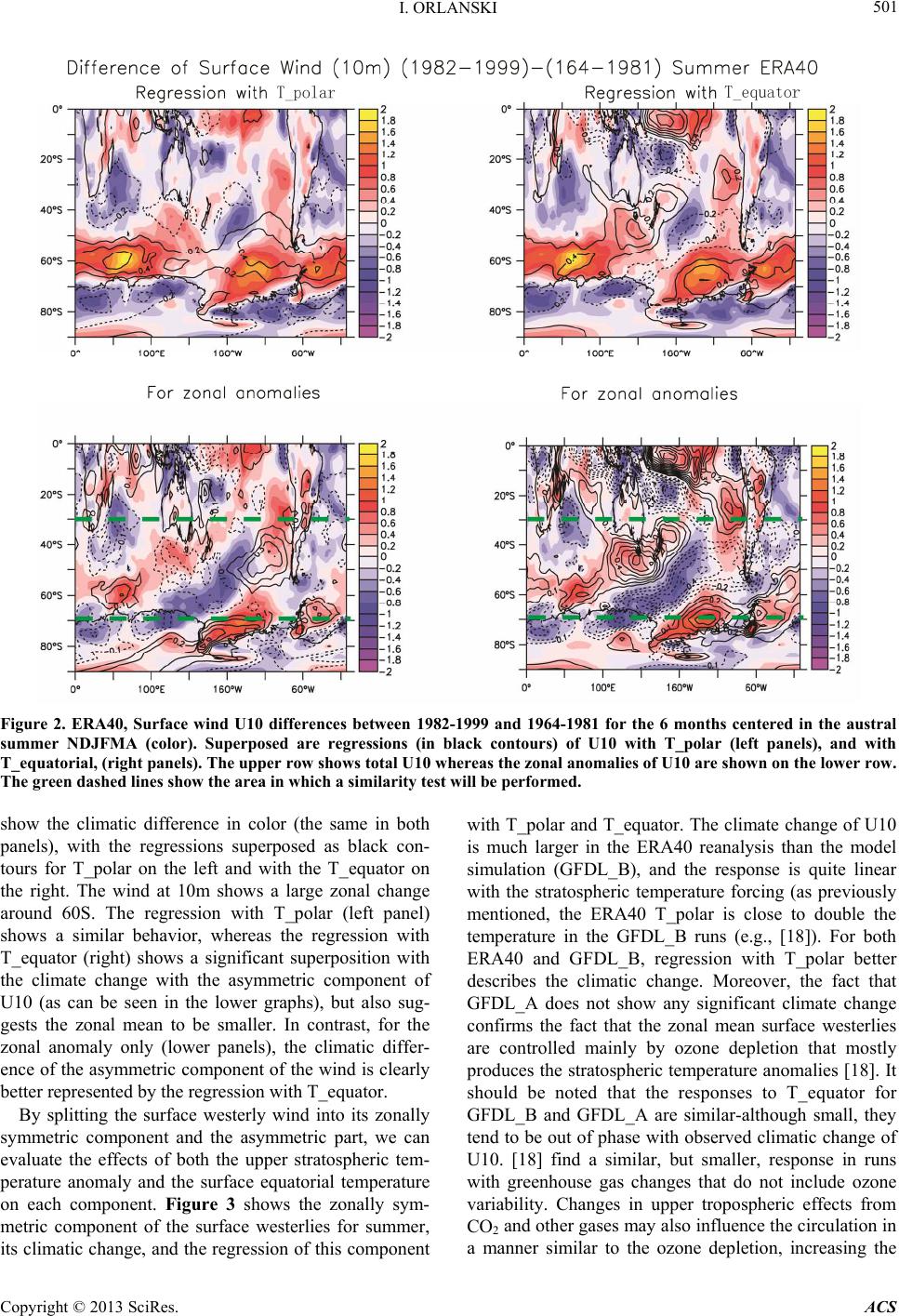

I. ORLANSKI 501
Figure 2. ERA40, Surface wind U10 differences between 1982-1999 and 1964-1981 for the 6 months centered in the austral
summer NDJFMA (color). Superposed are regressions (in black contours) of U10 with T_polar (left panels), and with
T_equatorial, (right panels). The upper row shows total U10 whereas the zonal anomalies of U10 are shown on the lower row.
The green dashed lines show the area in which a similarity test will be performed.
show the climatic difference in color (the same in both
panels), with the regressions superposed as black con-
tours for T_polar on the left and with the T_equator on
the right. The wind at 10m shows a large zonal change
around 60S. The regression with T_polar (left panel)
shows a similar behavior, whereas the regression with
T_equator (right) shows a significant superposition with
the climate change with the asymmetric component of
U10 (as can be seen in the lower graphs), but also sug-
gests the zonal mean to be smaller. In contrast, for the
zonal anomaly only (lower panels), the climatic differ-
ence of the asymmetric component of the wind is clearly
better represented by the regression with T_equator.
By splitting the surface westerly wind into its zonally
symmetric component and the asymmetric part, we can
evaluate the effects of both the upper stratospheric tem-
perature anomaly and the surface equatorial temperature
on each component. Figure 3 shows the zonally sym-
metric component of the surface westerlies for summer,
its climatic change, and the regression of this component
with T_polar and T_equator. The climate change of U10
is much larger in the ERA40 reanalysis than the model
simulation (GFDL_B), and the response is quite linear
with the stratospheric temperature forcing (as previously
mentioned, the ERA40 T_polar is close to double the
temperature in the GFDL_B runs (e.g., [18]). For both
ERA40 and GFDL_B, regression with T_polar better
describes the climatic change. Moreover, the fact that
GFDL_A does not show any significant climate change
confirms the fact that the zonal mean surface westerlies
are controlled mainly by ozone depletion that mostly
produces the stratospheric temperature anomalies [18]. It
should be noted that the responses to T_equator for
GFDL_B and GFDL_A are similar-although small, they
tend to be out of phase with observed climatic change of
U10. [18] find a similar, but smaller, response in runs
with greenhouse gas changes that do not include ozone
variability. Changes in upper tropospheric effects from
CO2 and other gases may also influence the circulation in
a manner similar to the ozone depletion, increasing the

I. ORLANSKI
502
Symmetric Componment of U10, Summer (NDJFMA)
Figure 3. Zonal average of U10, for the summer period. The
eighteen year difference (black) and both the regressions:
with T_polar (in blue) and T_equator (in red). The upper
panel is for ERA40, the middle panel for GFDL_B, and the
lower panel for GFDL_A.
surface zonal winds in sub-polar latitudes (as pointed out
by [18], to a much weaker degree than the effect of
ozone trends).
3.2. Changes in the Asymmetric Component of
U10
The asymmetric component of U10 for summer, shown
in the lower row of Figure 2, shows a very strong simi-
larity between the climatic change and the regression
with T_equator. It seems that, in the summer season, the
zonally symmetric component is controlled more by
variability in T_polar, whereas the asymmetric compo-
nent is explained by the regression with T_equator. In
order to quantify the role of each regression in explaining
the climatic difference patterns, we define a control pa-
rameter. This control parameter is defined as the positive
correlation between the difference pattern and the regres-
sion pattern over a specific region (in particular from 30S
to 70S shown as green dashed lines in Figure 2). Before
showing the correlation, let us review the patterns for the
winter season shown in Figure 4. As previously men-
tioned the total U10 in winter, exhibits large positive and
negative regions, but a small zonally symmetric compo-
nent. The asymmetric anomaly seems as large as in the
summer months. Again the most relevant feature is the
coherence between the climatic difference anomaly and
the regression with T_equator.
We can summarize the results by calculating the cor-
relation between the two regressions and the climatic
difference over the area shown between the green lines of
Figure 2. The control parameters for summer and winter
are shown in Figure 5 for the three data sets. There is
great consistency between the reanalysis and the two
model solutions. The outlier seems to be GFDL_B for
the summer season, but in general there is a very good
agreement among the figures, particularly for the winter
season. The averaged calculated correlation for each
member that composed the ensemble (Figure 5) of
GFDL_B runs is shown in Table 1. Values for GFDL_A
are not shown since only one major forcing was acting
for that case Note that each individual correlation be-
tween the climate change and the regression is a non-
linear function for each independent member and its av-
erage may not coincide with the ensemble mean correla-
tion. The results are fairly consistent among the members.
Which is remarkable given that the forcing for stationary
waves in the South Hemisphere is very weak; as a con-
sequence the variability between each member is consid-
erable. Because these asymmetries in the surface west-
erly wind should also be manifested in height anomalies,
we next apply the same analysis to that field.
4. Asymmetric Component of the
Geo-Potential Heights 300 hPa
The climatic change of the zonal anomalies of the 300
hPa height field for the ERA40 and both GFDL simula-
tions are shown in Figure 6 for the summer season. As in
Figure 2, we show the climatic difference in both panels
for the same row and the two regressions of that field,
with T_polar on the left and T_equator on the right. The
main characteristic of the response seems to be a wave
train of Rossby waves that emanate from the Indian
Ocean and propagate south east of the Pacific Ocean that

I. ORLANSKI
503
Figure 4. The same as in Figure 2, but for the 6 months centered in the austral winter.
Control Diagram of Polar and Equatorial Temperatures on Heights.
Figure 5. The control diagram summarizing how much the regressions with T_polar (blue) and T_equator (red) explain the
climate differences for each season. Each dataset is shown as in Figure 3.

I. ORLANSKI
504
Figure 6. The zonal anomalies for the 300 hPa heights are shown for the summer period. The climate differences are shown in
color. As in Figure 2, the regressions of T_polar and T_equator are shown in black contour. The upper row is for ERA40, the
middle row for GFDL_B and the lower row for GFDL_A.
is clearly seen in the ERA40, but is more weakly exhib-
ited in the other two simulations. Note that while both
regressions reproduce some features of the difference
fields for the ERA40, the GFDL simulations tend to be
consistent with ERA40 for the regression with T_equator,
in particular a height anomaly center around 110W and
60S. This pattern also seems to be characteristic of an
interannual pattern known as the PSA [17]. A superficial
inspection suggests that the combination of both regres-
sions could describe the summer difference pattern well.
However, for the winter patterns shown in Figure 7, the
T_equator regression practically reproduces the entire-

I. ORLANSKI 505
Figure 7. The same as in Figure 6, but for the winter period.
difference pattern in the ERA40 reanalysis, and shows
weaker but still good correlation with the differences in
the two GFDL simulations. In contrast, the T_polar re-
gression tends to be quite out of phase with all three dif-
ference patterns.
The results of Figures 6 and 7 can be summarized by
calculating the correlation pattern as has been shown for
U10 (Figure 5). The control parameter shown in Figure
8 contains clearly what we have seen in the previous
figures. The control is shared between T_polar and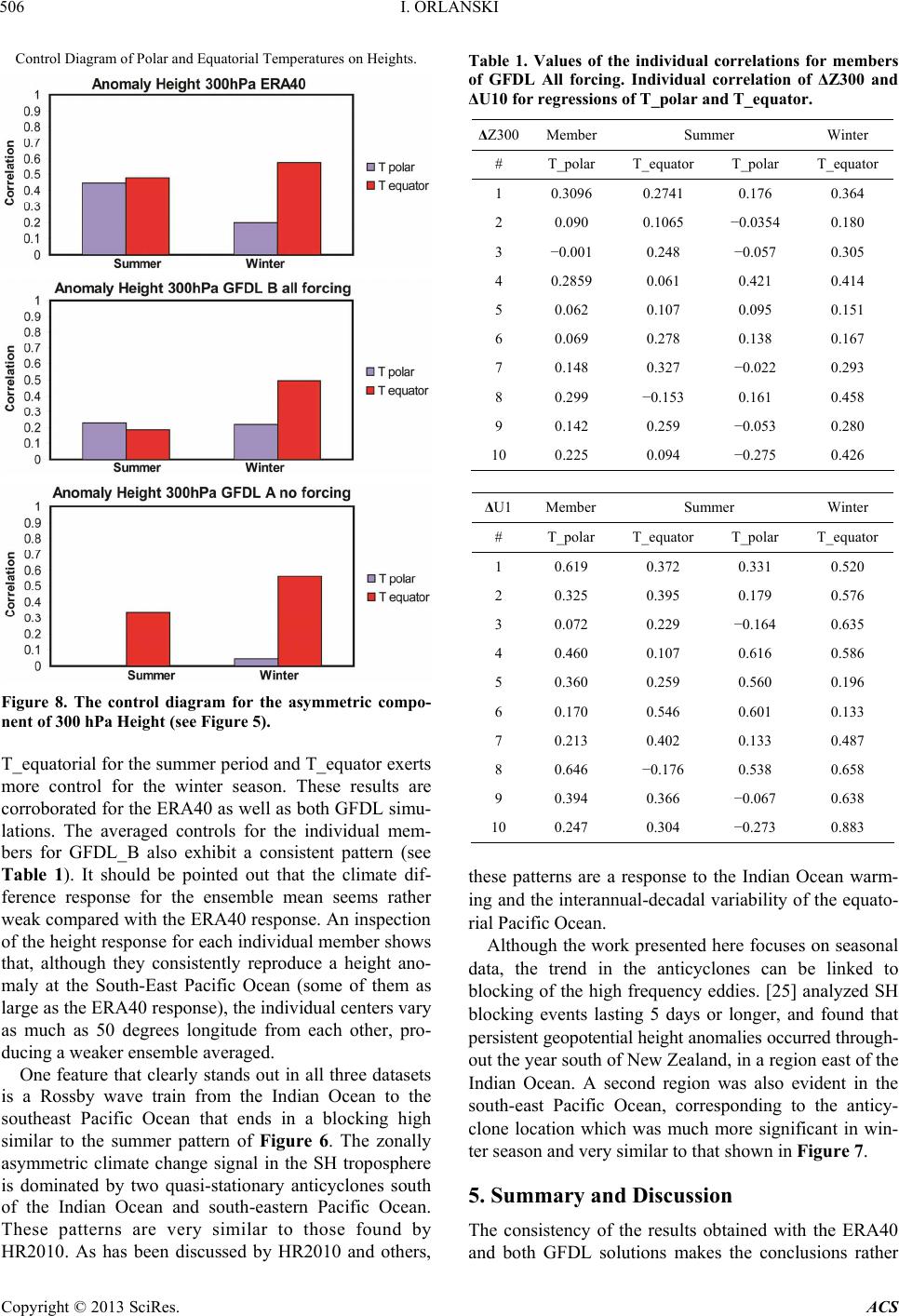

I. ORLANSKI
506
Control Diagram of Polar and Equatorial Temperatures on Heights.
Figure 8. The control diagram for the asymmetric compo-
nent of 300 hPa Height (see Figure 5).
T_equatorial for the summer period and T_equator exerts
more control for the winter season. These results are
corroborated for the ERA40 as well as both GFDL simu-
lations. The averaged controls for the individual mem-
bers for GFDL_B also exhibit a consistent pattern (see
Table 1). It should be pointed out that the climate dif-
ference response for the ensemble mean seems rather
weak compared with the ERA40 response. An inspection
of the height response for each individual member shows
that, although they consistently reproduce a height ano-
maly at the South-East Pacific Ocean (some of them as
large as the ERA40 response), the individual centers vary
as much as 50 degrees longitude from each other, pro-
ducing a weaker ensemble averaged.
One feature that clearly stands out in all three datasets
is a Rossby wave train from the Indian Ocean to the
southeast Pacific Ocean that ends in a blocking high
similar to the summer pattern of Figure 6. The zonally
asymmetric climate change signal in the SH troposphere
is dominated by two quasi-stationary anticyclones south
of the Indian Ocean and south-eastern Pacific Ocean.
These patterns are very similar to those found by
HR2010. As has been discussed by HR2010 and others,
Table 1. Values of the individual correlations for members
of GFDL All forcing. Individual correlation of ΔZ300 and
ΔU10 for regressions of T_polar and T_equator.
ΔZ300Member Summer Winter
# T_polar T_equator T_polar T_equator
1 0.3096 0.2741 0.176 0.364
2 0.090 0.1065 −0.0354 0.180
3 −0.001 0.248 −0.057 0.305
4 0.2859 0.061 0.421 0.414
5 0.062 0.107 0.095 0.151
6 0.069 0.278 0.138 0.167
7 0.148 0.327 −0.022 0.293
8 0.299 −0.153 0.161 0.458
9 0.142 0.259 −0.053 0.280
10 0.225 0.094 −0.275 0.426
ΔU1Member Summer Winter
# T_polar T_equator T_polar T_equator
1 0.619 0.372 0.331 0.520
2 0.325 0.395 0.179 0.576
3 0.072 0.229 −0.164 0.635
4 0.460 0.107 0.616 0.586
5 0.360 0.259 0.560 0.196
6 0.170 0.546 0.601 0.133
7 0.213 0.402 0.133 0.487
8 0.646 −0.176 0.538 0.658
9 0.394 0.366 −0.067 0.638
10 0.247 0.304 −0.273 0.883
these patterns are a response to the Indian Ocean warm-
ing and the interannual-decadal variability of the equato-
rial Pacific Ocean.
Although the work presented here focuses on seasonal
data, the trend in the anticyclones can be linked to
blocking of the high frequency eddies. [25] analyzed SH
blocking events lasting 5 days or longer, and found that
persistent geopotential height anomalies occurred through-
out the year south of New Zealand, in a region east of the
Indian Ocean. A second region was also evident in the
south-east Pacific Ocean, corresponding to the anticy-
clone location which was much more significant in win-
ter season and very similar to that shown in Figure 7.
5. Summary and Discussion
The consistency of the results obtained with the ERA40
and both GFDL solutions makes the conclusions rather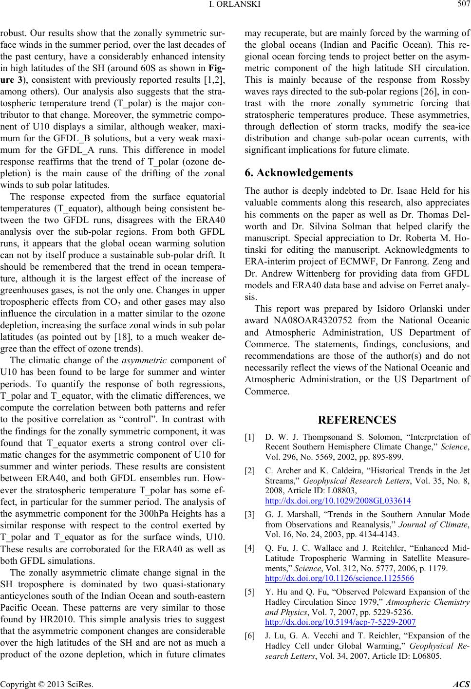

I. ORLANSKI 507
robust. Our results show that the zonally symmetric sur-
face winds in the summer period, over the last decades of
the past century, have a considerably enhanced intensity
in high latitudes of the SH (around 60S as shown in Fig-
ure 3), consistent with previously reported results [1,2],
among others). Our analysis also suggests that the stra-
tospheric temperature trend (T_polar) is the major con-
tributor to that change. Moreover, the symmetric compo-
nent of U10 displays a similar, although weaker, maxi-
mum for the GFDL_B solutions, but a very weak maxi-
mum for the GFDL_A runs. This difference in model
response reaffirms that the trend of T_polar (ozone de-
pletion) is the main cause of the drifting of the zonal
winds to sub polar latitudes.
The response expected from the surface equatorial
temperatures (T_equator), although being consistent be-
tween the two GFDL runs, disagrees with the ERA40
analysis over the sub-polar regions. From both GFDL
runs, it appears that the global ocean warming solution
can not by itself produce a sustainable sub-polar drift. It
should be remembered that the trend in ocean tempera-
ture, although it is the largest effect of the increase of
greenhouses gases, is not the only one. Changes in upper
tropospheric effects from CO2 and other gases may also
influence the circulation in a matter similar to the ozone
depletion, increasing the surface zonal winds in sub polar
latitudes (as pointed out by [18], to a much weaker de-
gree than the effect of ozone trends).
The climatic change of the asymmetric component of
U10 has been found to be large for summer and winter
periods. To quantify the response of both regressions,
T_polar and T_equator, with the climatic differences, we
compute the correlation between both patterns and refer
to the positive correlation as “control”. In contrast with
the findings for the zonally symmetric component, it was
found that T_equator exerts a strong control over cli-
matic changes for the asymmetric component of U10 for
summer and winter periods. These results are consistent
between ERA40, and both GFDL ensembles run. How-
ever the stratospheric temperature T_polar has some ef-
fect, in particular for the summer period. The analysis of
the asymmetric component for the 300hPa Heights has a
similar response with respect to the control exerted by
T_polar and T_equator as for the surface winds, U10.
These results are corroborated for the ERA40 as well as
both GFDL simulations.
The zonally asymmetric climate change signal in the
SH troposphere is dominated by two quasi-stationary
anticyclones south of the Indian Ocean and south-eastern
Pacific Ocean. These patterns are very similar to those
found by HR2010. This simple analysis tries to suggest
that the asymmetric component changes are considerable
over the high latitudes of the SH and are not as much a
product of the ozone depletion, which in future climates
may recuperate, but are mainly forced by the warming of
the global oceans (Indian and Pacific Ocean). This re-
gional ocean forcing tends to project better on the asym-
metric component of the high latitude SH circulation.
This is mainly because of the response from Rossby
waves rays directed to the sub-polar regions [26], in con-
trast with the more zonally symmetric forcing that
stratospheric temperatures produce. These asymmetries,
through deflection of storm tracks, modify the sea-ice
distribution and change sub-polar ocean currents, with
significant implications for future climate.
6. Acknowledgements
The author is deeply indebted to Dr. Isaac Held for his
valuable comments along this research, also appreciates
his comments on the paper as well as Dr. Thomas Del-
worth and Dr. Silvina Solman that helped clarify the
manuscript. Special appreciation to Dr. Roberta M. Ho-
tinski for editing the manuscript. Acknowledgments to
ERA-interim project of ECMWF, Dr Fanrong. Zeng and
Dr. Andrew Wittenberg for providing data from GFDL
models and ERA40 data base and advise on Ferret analy-
sis.
This report was prepared by Isidoro Orlanski under
award NA08OAR4320752 from the National Oceanic
and Atmospheric Administration, US Department of
Commerce. The statements, findings, conclusions, and
recommendations are those of the author(s) and do not
necessarily reflect the views of the National Oceanic and
Atmospheric Administration, or the US Department of
Commerce.
REFERENCES
[1] D. W. J. Thompsonand S. Solomon, “Interpretation of
Recent Southern Hemisphere Climate Change,” Science,
Vol. 296, No. 5569, 2002, pp. 895-899.
[2] C. Archer and K. Caldeira, “Historical Trends in the Jet
Streams,” Geophysical Research Letters, Vol. 35, No. 8,
2008, Article ID: L08803,
http://dx.doi.org/10.1029/2008GL033614
[3] G. J. Marshall, “Trends in the Southern Annular Mode
from Observations and Reanalysis,” Journal of Climate,
Vol. 16, No. 24, 2003, pp. 4134-4143.
[4] Q. Fu, J. C. Wallace and J. Reitchler, “Enhanced Mid-
Latitude Tropospheric Warming in Satellite Measure-
ments,” Science, Vol. 312, No. 5777, 2006, p. 1179.
http://dx.doi.org/10.1126/science.1125566
[5] Y. Hu and Q. Fu, “Observed Poleward Expansion of the
Hadley Circulation Since 1979,” Atmospheric Chemistry
and Physics, Vol. 7, 2007, pp. 5229-5236.
http://dx.doi.org/10.5194/acp-7-5229-2007
[6] J. Lu, G. A. Vecchi and T. Reichler, “Expansion of the
Hadley Cell under Global Warming,” Geophysical Re-
search Letters, Vol. 34, 2007, Article ID: L06805.

I. ORLANSKI
508
http://dx.doi.org/10.1029/2006GL028443
[7] C. Vera, G. Silvestri, B. Liebmann and P. Gonzalez,
“Climate Change Scenarios for Seasonal Precipitacion in
South America from IPCC-AR4 Models,” Geophysical
Research Letters, Vol. 33, 2006, Article ID: L13707.
[8] S. Solman and I. Orlanski, “Subpolar High Anomaly Pre-
conditioning Precipitation over South America,” Journal
of the Atmospheric Sciences, Vol. 67, No. 5, 2010, pp.
1526-1542. http://dx.doi.org/10.1175/2009JAS3309.1
[9] B. L. Preston and R. N. Jones, “Climate Change Impacts
on Australia and the Benefits of Early Action to Reduce
Global Greenhouse Gas Emissions,” Report CSIRO, 2006.
[10] H. D. Pritchard, et al., “Antarctic Ice-Sheet Loss Driven
by Basal Melting of Ice Shelves,” Nature, Vol. 484, 2012,
pp. 502-505. http://dx.doi.org/10.1038/nature10968
[11] D. G. Vaughn, G. J. Marshall, W. M. Connolley, C. Park-
inson, R. Mulvaney, D. A. Hodgson, J. C. King, J. C.
Pudsey and J. Turner, “Recent Rapid Regional Climate
Warming in the Antarctic Peninsula,” Climate Change,
Vol. 60, 2003, pp. 243-274.
[12] J. Turner and J. Overland, “Contrasting Climate Change
in the Two Polar Regions,” Polar Research, Vol. 28, No.
2, 2009, pp. 146-164.
http://dx.doi.org/10.1111/j.1751-8369.2009.00128.x
[13] J. Turner, T. A. Lachlan-Cope, S. Colwell, G. J. Marshall
and W. M. Connolley, “Significant Warming of the Ant-
arctic Winter Troposphere,” Science, Vol. 311, No. 5769,
2006, pp. 1914-1917.
http://dx.doi.org/10.1126/science.1121652
[14] E. J. Steig, D. P. Schneider, S. D. Rutherford, M. E.
Mann, J. C. Comiso and D. T. Shindell, “Warming of the
Antarctic Ice-Sheet Surface Since the 1957 International
Geophysical Year,” Nature, Vol. 1457, No. 7228, 2009, pp.
459-463. http://dx.doi.org/10.1038/nature07669
[15] R. W. Hobbs and M. N. Raphael, “Characterizing the
Zonally Asymmetric Component of the SH Circulation,”
Climate Dynamics, Vol. 35, 2010, pp. 859-873.
[16] N. Mathewman and G. Magnusdottir, “Clarifying Ambi-
guity in Intraseasonal Sothern Hemisphere Climate
Modes during Austral Winter,” Journal of Geophysical
Research, Vol. 113, No. D7, 2012, Article ID: D03105.
[17] K. C. Mo and J. N. Paegle, “The Pacific-South American
Modes and Their Downstream Effects,” International Jour-
nal of Climatology, Vol. 21, No. 10, 2001, pp. 1211-1229.
[18] L.-M. Polvani, D. W. Waugh, G. J. P. Correa and S.-W.
Son, “Stratospheric Ozone Depletion: The Main Driver of
Twentieth-Century Atmospheric Ciruclation Changes in
the Southern Hemisphere,” Journal of Climate, Vol. 24,
2011, pp. 795-812.
[19] S. M. Uppala, et al., “The ERA-40 Re-Analysis,” Quar-
terly Journal of the Royal Meteorological Society, Vol.
131, 2005, pp. 2961-3012.
[20] J. Anderson, et al., “The New GFDL Global Atmosphere
and Landmodel AM2/LM2: Evaluation with Prescribed
SST Simulations,” Journal of Climate, Vol. 17, 2004, pp.
4641-4673.
[21] D. W. J. Thompson, J. M. Wallace and G. C. Hegerl,
“Annular Modes in the Extra-Tropical Circulation, Part II:
Trends,” Journal of Climate, Vol. 13, 2000, p. 1018.
[22] L. Polvani and P. J. Kushner, “Tropospheric Response to
Stratospheric Perturbations in a Relatively Simple Gen-
eral Circulation Model,” Geophysical Research Letters,
Vol. 29, No. 7, 2002, 18 p.
http://dx.doi.org/10.1029/2001GL014284
[23] G. Chen and I. M. Held, “Phase Speed Spectra and the
Recent Poleward Shift of Southern Hemisphere Surface
Westerlies,” Geophysical Research Letters, Vol. 34, No.
21, 2007, Article ID: L21805.
http://dx.doi.org/10.1029/2007GL031200
[24] P. Kushner, I. M. Held and T. L. Delworth, “Southern
Hemisphere Atmospheric Circulation Response to Global
Warming,” Journal of Climate, Vol. 14, No. 10, 2001, pp.
2238-2249.
http://dx.doi.org/10.1175/1520-0442(2001)014<0001:SH
ACRT>2.0.CO;2
[25] K. E. Trenberth and K. C. Mo, “Blocking in the Southern
Hemisphere,” Monthly Weather Review, Vol. 113, No. 1,
1985, pp. 3-21.
[26] I. Orlanski and S. Solman, “The Mutual Interaction be-
tween External Rossby Waves and Thermal Forcing: The
Sub-Polar Region,” Journal of the Atmospheric Sciences,
Vol. 67, 2010, pp. 2018-2038.

I. ORLANSKI 509
Appendix
To Partially Decorrelate the Time Series
Assume two time series that are slightly correlated, say:


YYt and


TTt A1
The cross-correlation between them is:





1
YTY T
CYTN 
  
 A2
where Y

, T

are the standard deviations of each function.




0.5
21
UUŪN
  
 A3
where Ū is the mean of the variable U.
To decorrelate Y with T, it is enough to calculate the regression of Y on T as follows:





1
Y
RYTN 
  
T
A4
Then the decorrelated Y anomaly can be written as:
dcY T
YYRT




 A6
It is easy to see the correlation between T' and dc Y

is equal to zero. However it seems asymmetric: one time series
has been modified and the other not. We could apply the same algorithm to both time series to partially decorrelate
them. In this case, the correlation between
dc
Ydc T

is not zero, but it is very small.
0.5
dcY T
YY RT




 A7
T TT0.5**T
dc T
R




 A8
 


 


22
1
0.25 0.51
Y
YdcTdcdcdcYdc Tdc
TYTY TYdcTdcTT
CYTN
YTRRYTRY RYN

 

 

   


 A9
Replacing RT and RY for their definition A4, it is easy to show that the last term of A9 can be written as follows:




22
0.5 TYTT RYRYY T 






A10
And the expression in A9 can be reduced to:






0.251
YYdcTdcTYYdc TdcT
CRRYTN  

 

A11
Recognizing that the Standard deviation Ydc

and Tdc

can be rewritten as:





22
0.25 1
TYdcYY T
YRYR NTT  
 





A12
Using the definitions A2, A3 and A4, A12 can be written as follows:

0.5
2
10.75
Ydc YYT
C  
And similarly for: A13
(A13)

0.5
2
10.75
Tdc TYT
C  
Finally, the correlation of the partially decorrelated time series A7-A8



32
0.251 0.75
YdcTdc YTYT
CC C A14
shows that for cases in which CYT ~ −0.3, as in our case,
0.0072
YdcTdc
C


the time series is very well decorrelated.
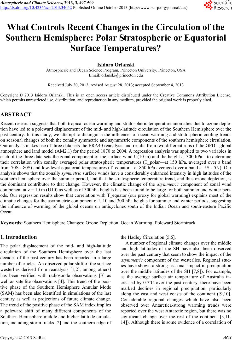