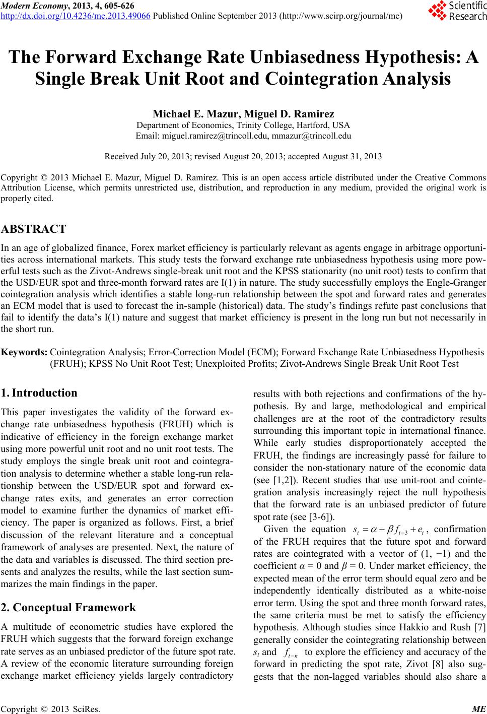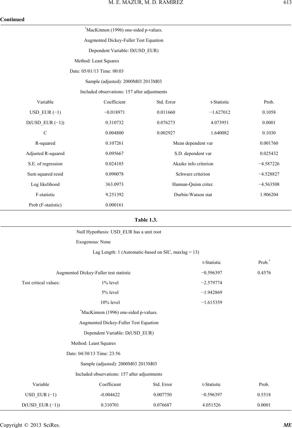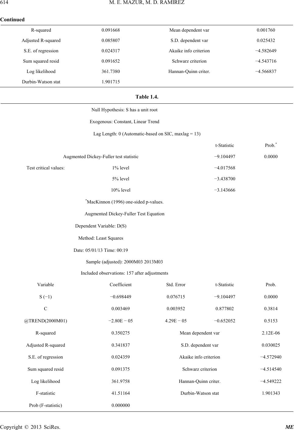
M. E. MAZUR, M. D. RAMIREZ
610
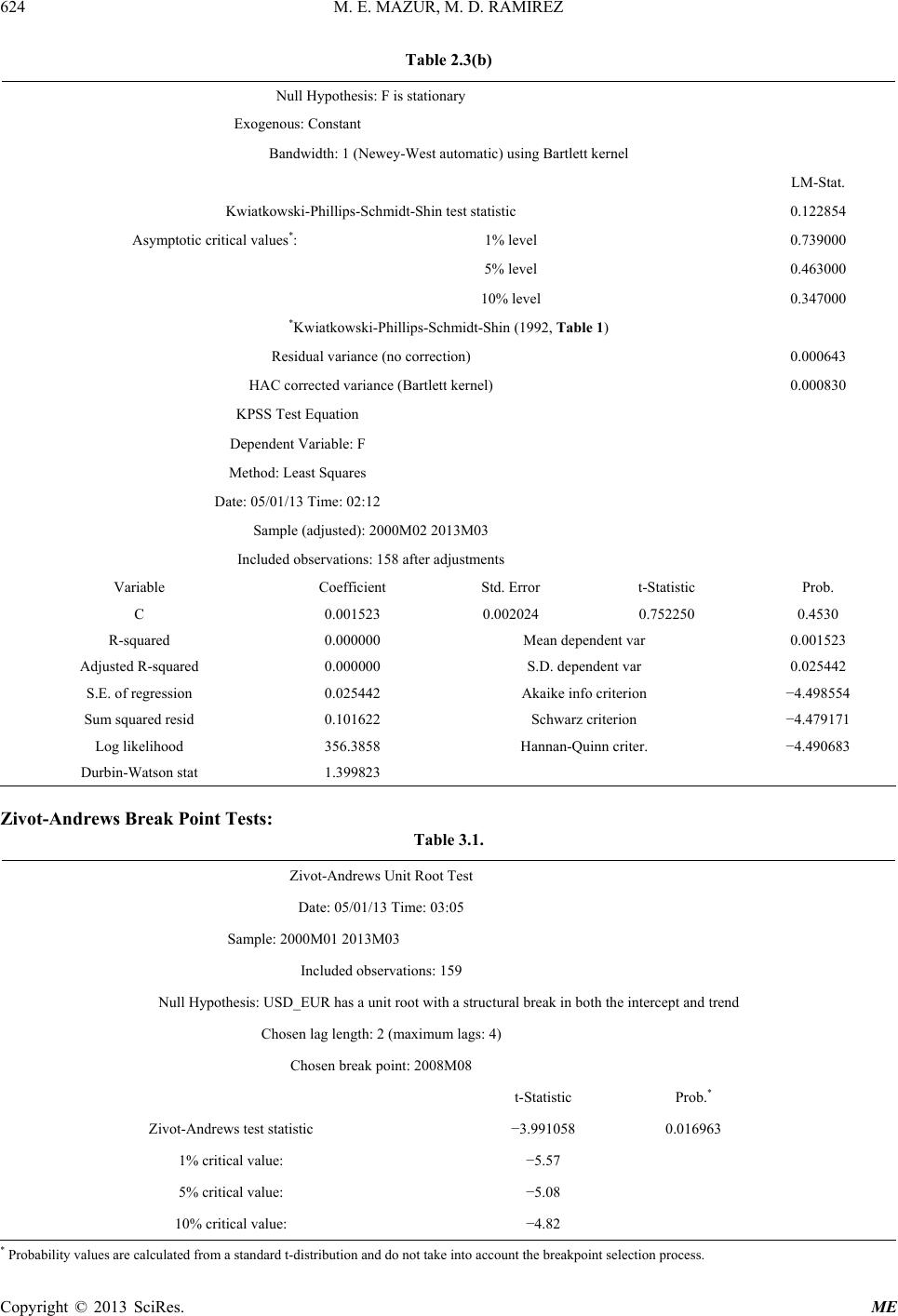
Figure 4. Theil inequality coefficient for in-sample forecast.
proportion should equal one. The reported estimates su-
ggest that all of these ratios are close to their optimum
values (bias = 0.0000, variance = 0.0067, and covariance
= 0.9932). Sensitivity analysis on the coefficients also
revealed that changes in the initial or ending period did
not alter the predictive power of the selected models (re-
sults are available upon request).
5. Conclusion
Efficiency in the foreign exchange market is especially
relevant in the world of globalized finance since market
agents are frequently and increasingly transacting both at
home and abroad. This study shows that the spot and
three-month forward exchange rates are I(1) processes
using the more powerful KPPS stationarity test and the
Zivot Andrews single break unit root test. Following the
Engle-Granger cointegration analysis framework, a long-
run stable relationship between the three-month forward
exchange rate and the future spot rate is identified which
suggests that the forward rate contains useful information
about the spot rate; in other words, it supports market
efficiency in the long run. Insofar as the error correction
model is concerned, it provided further support for the
forward exchange rate unbiasedness hypothesis. With a
high degree of power, the results of the model fulfill the
final two criteria for market efficiency, viz., a constant
equal to 0 and a coefficient of 1. However, the results
also suggest that there is a disequilibrium in the short run
that is only partially corrected in subsequent periods,
suggesting that, in the short run, there might be unex-
ploited profit opportunities for speculators and/or a time-
varying risk premium. Needless to say, economists have
debated the issue of exchange market efficiency since the
70’s and this study, although supportive of market effi-
ciency in the long run, will by no means settle the con-
troversy. Finally, the endogenously determined structural
breaks in the data indicate that, since the common cur-
rency’s inception, volatility and disruption of the Forex
market have been generated by both the un-expected
costs associated with the war in Iraq and the 2008 global
financial crisis.
REFERENCES
[1] R. M. Levich, “Empirical Studies of Exchange Rates,
Price Behavior, Rate Determination, and Market Effi-
ciency,” In: R. W. Jones and P. B. Kennen, Eds., Hand-
book of International Economics, Vol. II, Elsevier, Am-
sterdam, 1978, pp. 979-1040.
[2] J. A. Frenkel, “Flexible Exchange Rates, Prices, and the
Role of News: Lessons from the 1970s,” In: R. A. Bat-
chelor and G. E. Wood, Eds., Exchange Rate Policy, Ma-
cmillan, London, 1982.
[3] R. E. Cumby and M. Obstfeld, “International Interest
Rate and Price Level Linkages under Flexible Exchange
Rates: A Review of the Evidence,” 1984.
[4] C. Engel, “The Forward Discount Anomaly and the Risk
Premium: A Survey of Recent Evidence,” Journal of Em-
pirical Finance, Vol. 3, No. 2, 1996, pp. 123-192.
[5] J. Olmo and K. Pilbeam, “Uncovered Interest Parity and
the Efficiency of the Foreign Exchange Market: A Re-
examination of the Evidence,” International Journal of
Finance and Economics, Vol. 16, No. 2, 2011, pp. 189-
204. doi:10.1002/ijfe.429
[6] V. Ukpolo, “Exchange Rate Market Efficiency; Further
Evidence from Cointegration Tests,” Applied Economics
Letters, Vol. 2, No. 6, 1995, pp. 196-198.
doi:10.1080/135048595357438
[7] C. S. Hakkio and M. Rush, “Cointegration: How Short Is
the Long Run?” Journal of International Money and Fi-
nance, Vol. 10, No. 4, 1991, pp. 571-581.
doi:10.1016/0261-5606(91)90008-8
[8] E. Zivot, “Cointegration and Forward and Spot Exchange
Rate Regressions,” 1998.
http://128.118.178.162/eps/em/papers/9812/9812001.pdf
[9] M. Kuhl, “Cointegration in the Foreign Exchange Market
and Market Efficiency since the Introduction of the Euro:
Evidence Based on bivariate Cointegration Analyses,”
2007.
[10] D. W. Duisenberg, “Recent Developments and Trends in
World Financial Market,” 2000.
http://www.ecb.int/press/key/date/2000/html/sp001114.en
.html
[11] A. C. Jung and V. Wieland, “Forward Rates and Spot
Rates in the European Monetary System-Forward Market
Efficiency,” Weltwirtschaftliches Archiv, Vol. 126, No. 4,
1990, pp. 615-629. doi:10.1007/BF02707471
[12] E. Zivot and D. Andrews, “Further Evidence of Great
Crash, the Oil Price Shock, and Unit Root Hypothesis,”
Journal of Business and Economic Statistics, Vol. 10, No.
3, 1992, pp. 251-270.
doi:10.1080/07350015.1992.10509904
[13] D. Kwaitkowski, P. C. B. Phillips, P. Schmidt and Y.
Shin, “Testing the Null Hypothesis of Stationarity against
the Alternative of a Unit Root,” Journal of Econometrics,
Vol. 54, No. 1-3, 1992, pp. 159-178.
doi:10.1016/0304-4076(92)90104-Y
[14] P. Perron, “The Great Crash, the Oil Price Shock and the
Unit Root Hypothesis,” Econometrica, Vol. 57, No. 6,
1989, pp. 1361-1401. doi:10.2307/1913712
[15] A. Seton, “On Unit Root Tests when the Alternative Is a
Copyright © 2013 SciRes. ME