American Journal of Computational Mathematics, 2013, 3, 242-251
http://dx.doi.org/10.4236/ajcm.2013.33034 Published Online September 2013 (http://www.scirp.org/journal/ajcm)
Enhanced Frequency Resolution in Data Analysis
Luca Perotti, Daniel Vrinceanu, Daniel Bessis
Department of Physics, Texas Southern University, Houston, USA
Received March 14, 2013; revised May 8, 2013; accepted July 9, 2013
Copyright © 2013 Luca Perotti et al. This is an open access article distributed under the Creative Commons Attribution License,
which permits unrestricted use, distribution, and reproduction in any medium, provided the original work is properly cited.
ABSTRACT
We present a numerical study of the resolution power of Padé Approximations to the Z-transform, compared to the Fou-
rier transform. As signals are represented as isolated poles of the Padé Approximant to the Z-transform, resolution de-
pends on the relative position of signal poles in the com plex plane i.e. not only the difference in frequency (separation
in angular position) but also the difference in the decay constant (separation in radial position) contributes to the reso-
lution. The frequency resolution increase reported by other authors is therefore an upper limit: in the case of signals
with different dec ay rates frequency resolution can be further increased.
Keywords: Frequency Resolution; Z-Transform; Padé Approximations
1. Introduction
It is known that Padé app roximants to the Z-transform of
a time series allow “super resolution” of signals in low
noise: for instance, when the signal to noise ratio (SNR)
is high enough (more than 105) we can resolve frequencies
separated by 4max 10 f
 with less than 100 data po-
ints: better than discre te Fourier Transfo rm ( D FT ) i n
the same noise conditions. This property has been ob-
served both by P. Barone [ 1 , 2] and D. Belkich [3].
2
10
Up to now no extensive study has been made of this
remarkable property of Padé approximants, not only
concerning the limits of super resolution but also of the
implications of why it is so.
The key point we want to address in the present note is
that resolution for Padé approximants is in the complex
plane, not in frequency alone as is in the case of DFT.
This allows not only even better frequency resolutions of
those reported above, when the decay rates of neighbouring
peaks are different, but also resolution of wide overlap-
ping peaks .
Given a data series 012 ,,, ,
N
s
ss s, its “Z-transform”
is:

0
;
Ni
i
i
Z
zsz


 (1)
DFT is clearly the “Z-transform” calculated on the
roots of unity. This means that DFT has two
intrinsic limitations.
1N
1) There is a resolution limit, due to the time of
observation:
Let
T
be the total sampling time and N the number
of sampled points; the time step will be TN ; the
maximum detectable frequency will therefore be
max 12 2fNT

 and the frequency step (resolution)
11
fNT

.
Scaling to the unit circle where the roots of unity
reside , max
f
becomes 12 the frequency st ep is t her efore
max
..
ff
UC 21
f
N.


This is the well known Nyquist limit [4]. The Padé ap-
proximation to the “Z-transform” is supperior to it through
nonlinearity: because of its discreteness, the average den-
sity of peaks is the same as for the DFT; but while the
local density in DFT is the same as the av erag e density, it
can be very different when a Padé analysis is used, since
its peaks are not bound to fall on the regu lar lattice of the
roots of unity. This is the source of “super resolu tion” for
constant amplitude signals reported in the papers men-
tioned above.
2) Damped signals have a natural width on the unit
circle.
The peak for a damped signal is a Lorentzian of the
form


2
2
20
I
F

  (2)
where
I
is the height of the peak,

is the decay
factor and 2
f


. The half height width is therefore
2W



or f W


. Scaling to the unit circle, max
f
C
opyright © 2013 SciRes. AJCM

L. PEROTTI ET AL. 243
becomes 12. The width is therefore
.. max
2
UC f
WWf

 where

 is the
dimensionless decay factor.
This means that, when using the Fourier Transform,
increasing numerical resolution (sampling rate) beyond
the natural linewidth of the signals involved is not much
use in separating neighbouring peaks.
When using the Padé Approximant approach, things
are very different: signals are represented by poles in the
complex plane and all poles are by definition singulari-
ties of Z(z) and therefore sharp. The basic point is that
poles corresponding to damped signals are off the unit
circle and are sharp only if we look at them in the
complex plane; if we only loo k on the unit circle, as it is
the case when using DFT, we do not see the singularity
itself but the profile of its tail as the intersection of Z(z)
with the unit circle.
This has two consequences:
1) as we are looking at the poles themselves, there are
no tails of strong wide peaks that can hide nearby peaks.
2) Since what counts is the distance of neighbouring
peaks in the comp lex plane, damped signals can be even
closer in frequency than reported above if their damping
constants (radial positions) are different.
2. Summary of the Method
Given a data series 012 ,,, ,
N
s
ss s
N
N
, we build its generat-
ing function, or “Z-transform” Equation 1 and construct
its diagonal Padé Approximant, i.e. a rational function
with the numerator and denominator having the same
degree and whose Taylor expansion equals the Z-trans-
form up to order . The aim is to try and predict the
“Z-transform” for .
The choice of a diagonal rational approximation is the
best for both signal and noise because of the following
considerations.
For a finite ensemble of damped oscillators, the Z-
transform tends, when the number of data points goes to
infinity, to a


nn rational function in z, with 2nN

equal to twice the number of oscillators [5]. A diagonal
Padé Approximant therefore has the right structure for
the signal.
For pure noise, the organization of poles and zeros in
Froissart doublets [6-9] is again best approximated by a


nn rational function in
z
.
Most data analysts stopped using Padé Approximants
because of instabilities due to the fact that for a pure
signal, singularities appear when one tries to construct a
Padé Approximant of order higher than


nn. The prob-
lem is conveniently solved by the presence of noise who s e
Froissart doublets act as additional “signals”.
To numerically calculate poles and zeros of the Padé
Approximant of the Z-transform of a finite time series,
we build directly from the time series two tridiagonal
Hilbert space operators, called J-Matrices, one for the
numerator and one for the denominator. The eigenvalues
of these matrices readily provide the desired zeros and
poles. Details of our method can be found in [5]. Knowl-
edge of the positions of all poles and zeros also gives us
the residues for all poles and therefore the amplitudes
and phases of the signal oscillations.
3. Results and Sensitivity of the Method
When dealing with resolution, key parameters for both
Padé Approximant and Fourier Transform are:
1) the angular distance of the two signal poles, i.e. the
frequency difference scaled to the maximum detectable
frequency: this is the resolution itself.
2) The radial position

of the two signal poles, i.e.
the decay factor ln


 of each of the signals.
3) The relative amplitude of the two signals.
4) The signal to noise ratio of the smaller of the two
signals, or equivalently , its precision in num ber of digits.
5) The number of data poin ts.
These are the factors that in practice can limit resolu-
tion, which assuming infinite data precision and arbitrar-
ily small noise has no limitatio n for Padé Approximants.
We now pass to look at a few cases that can help
clarify how parameters 2, 3, 4 and 5 affect resolution.
3.1. Two Equal Peaks on the Unit Circle
As a first example, let us consider two peaks on the unit
circle separated by along the circumference,
i.e. two constant amplitude waves whose frequency dif-
ference is
3
410 


max
2
3
410
f

. Using the DFT to resolve them
we need a frequency step at least half the distance, i.e.
3
.. 410 2
fUC


3
10N
, which means a number of data poin ts
.
Figure 1 shows what can be seen with 256N

data
points. By increasing N to (Figure 2) a de-
cent resolution can be obtained. 8192N
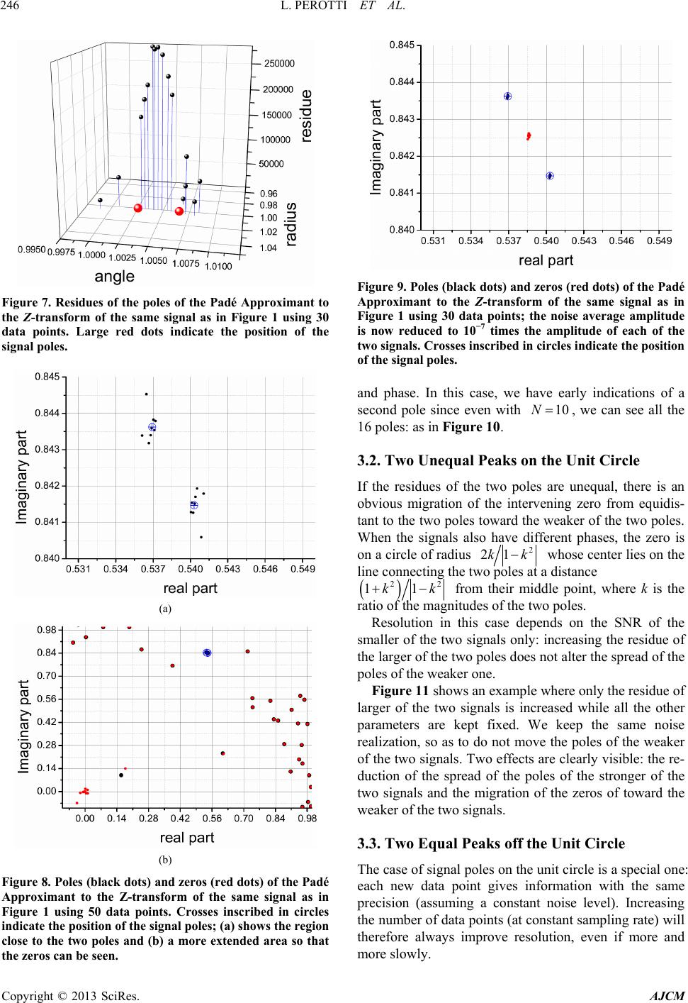
Assuming the noise average amplitude to be 10–5 times
the amplitude of each of the two signals, and assuming
the data to be in double precision, the diagonal Padé
Approximant instead need s only 40 data points to resolve
the two signals with reasonable accuracy; a reduction by
two orders of magnitude. Figure 3 shows the positions
and residues of the reconstructed signal poles for 8
different realizations of the noise: there is some spread in
position and amplitude (pole residue) which completely
disappears by doublin g th e nu mber of d ata p oints, bu t the
16 poles are clearly grouped around the positions of the
two input poles marked by large red dots. 8 zeros fall
between the two groups of poles. The resolution transi-
tion between 1 and 2 signals takes place as follows. For
low only 8 poles with sizable residues are visible,
one for each noise realization, clustered halfway between
the positions of the two signal p oles; Figure 4 shows th e
N

L. PEROTTI ET AL.
244
Figure 1. FFT for a signal corresponding to two peaks on
the unit circle distant using 256 data points.
The noise average amplitude is 10−5 times the amplitude of
each of the two signals.


 3 4 10
Figure 2. FFT for the same signal as in Figure 1 using 8192
data points.
case for . The noise doublets are spread around
the unit circle away from the signal poles; we discussed
this repulsion in [10]. By increasing , we see that 8
doublets, one for each data sequence, approach the signal
poles, see Figure 5.
10N
N
Close to the signal poles the doublets split while the
central cluster of 8 poles also breaks up; finally the
poles regroup in the two clusters visible in Figure 3 with
the zeros halfway between them. Figure 6 shows this
sequence of events. Already for all 16 po les are
visible, even if the two clusters visible in Figure 3 are
not yet fully formed: see Figure 7.
30N
The case we have shown is that of equal phases of the
two signals; for different phases the zeros are on the
straight line perpendicular to the line connecting the two
poles and crossing it halfway between the two poles.
Figure 8 shows the case when the signal residues have
Figure 3. Residues of the poles of the Padé Approximant to
the Z-transform of the same signal as in Figure 1 using 40
data points. Large red dots indicate the position of the
signal poles.
Figure 4. Residues of the poles of the Padé Approximant to
the Z-transform of the same signal as in Figure 1 using only
10 data points. Large red dots indicate the position of the
signal poles.
opposite sign: no zero is present near the signal poles as
in Figure 8(a); all the zeros are clustered at the ori-
gin as in Figure 8(b). 8
Noise amplitude determines the number of data points
necessary to resolve two signals at a given distance: if we
reduce the noise level from to then
5
107 1030N

data points are again sufficient to get a very good reso-
lution. Figure 9 shows the positions of the poles (black
dots) and zeros (red dots) for 8 different realizations of
the noise: the spread of each cluster of poles is minimal
and all the zeros are located halfway between them
because the two signals have again the same amplitude

L. PEROTTI ET AL.
245
(a) (b)
Figure 5. Poles (black dots) and zeros (red dots) of the Padé Approximant to the Z-transform of the same signal as in Figure 1
using (a) 10 and (b) 20 data points. Crosses inscribed in circles indicate the position of the signal poles.
(a) (b)
(c) (d)
Figure 6. Poles (black dots) and zeros (red dots) of the Padé Approximant to the Z-transform of the same signal as in Figure 1
using (a) 20; (b) 30; (c) 40; and (d) 50 data points. Crosses inscribed in circles indicate the position of the signal poles.

L. PEROTTI ET AL.
246
Figure 7. Residues of the poles of the Padé Approximant to
the Z-transform of the same signal as in Figure 1 using 30
data points. Large red dots indicate the position of the
signal poles.
(a)
(b)
Figure 8. Poles (black dots) and zeros (red dots) of the Padé
Approximant to the Z-transform of the same signal as in
Figure 1 using 50 data points. Crosses inscribed in circles
indicate the position of the signal poles; (a) shows the region
close to the two poles and (b) a more extended area so that
the zeros can be seen.
Figure 9. Poles (black dots) and zeros (red dots) of the Padé
Approximant to the Z-transform of the same signal as in
Figure 1 using 30 data points; the noise average amplitude
is now reduced to 10−7 times the amplitude of each of the
two signals. Crosses inscribed in circles indicate the position
of the signal poles.
and phase. In this case, we have early indications of a
second pole since even with , we can see all the
16 poles: as in Figure 10. 10N
3.2. Two Unequal Peaks on the Unit Circle
If the residues of the two poles are unequal, there is an
obvious migration of the intervening zero from equidis-
tant to the two poles toward the weaker of the two poles.
When the signals also have different phases, the zero is
on a circle of radius 2
21kk whos e center lies o n th e
line connecting the two poles at a distance


2
11k
2
k from their middle point, where k is the
ratio of the magnitudes of the two po les.
Resolution in this case depends on the SNR of the
smaller of the two signals only: increasing the residue of
the larger of the two poles does not alter the spread of th e
poles of the weaker one.
Figure 11 shows an example where only the residue of
larger of the two signals is increased while all the other
parameters are kept fixed. We keep the same noise
realization, so as to do not move the poles of the weaker
of the two signals. Two effects are clearly visible: the re-
duction of the spread of the poles of the stronger of the
two signals and the migration of the zeros of toward the
weaker of the two signals.
3.3. Two Equal Peaks off the Unit Circle
The case of signal poles on the unit circle is a special one:
each new data point gives information with the same
precision (assuming a constant noise level). Increasing
the number of data points (at constant sampling rate) will
therefore always improve resolution, even if more and
more slowly.

L. PEROTTI ET AL. 247
Figure 10. Residues of the poles of the Padé Approximant to
the Z-transform of the same signal as in Figure 9 using 10
data points. Large red dots indicate the position of the
signal poles.
If it is possible to increase the sampling rate at will,
then—for any given decay time—the signal poles can be
moved as close as we want to the unit circle and we are
back to the unit circle case.
If instead the sampling rate is limited, then—for any
given distance between signal poles—we’ll have to
search for the optimal number of data points as a func-
tion not only of the SNR but also of the data poles
distance from the unit circle.
Signal poles off the unit circle correspond to damped
signals; again assuming constant noise amplitude (and
data precision) each new point will have lower and lower
precision. One might therefore expect (for a given noise
level and data precision) the resolution to first increase
and then decrease when increasing the number of data po-
ints. We do not have evidence of this kind of behaviour.
What we instead see is:
1) Compared to the unit circle case, a very slow resolu-
tio n increase with the number of points: for 5 noise 10

,
two peaks, radial position 0.95


, angle 1.0


, and
separation , not much difference is seen
going from 100 (Figure 12(a)) to 200 (Figure 12(b))
data points.
3
410 


2) A decrease of resolution when moving off the unit
circle: in the case of two peaks, angle 1.0

, and sepa-
ration , going from the unit circle to a radial
position
3
410 


0.95

, noise has to be reduced from 5 10

to to get a comparable resolution with 300 data
points: see Figure 13.
7
10
3) The relevant distance is not the frequency one, but
the one in the complex plane. For example, for
, two peaks, radial position ρ = 0.950, angle
φ = 1.000, separation , and N = 300, there is
no relevant difference in the spread of the signal poles
5
noise 10 3
410 


(a)
(b)
(c)
Figure 11. Poles (black dots) and zeros (red dots) of the
Padé Approximant to the Z-transform of two signals on the
unit circle distant using 50 data points. The
noise average amplitude is 10−5 times the amplitude of the
residue of the weaker pole. (a) Equal residues; (b) Second
pole twice as big as the first one; (c) Second pole 100 times
bigger than the first one; Crosses inscribed in circles indicate
the position of the signal poles.


 3 4 10

L. PEROTTI ET AL.
248
(a)
(b)
Figure 12. Residues of the poles of the Padé Approximant to
the Z-transform of the signal generated by 2 poles in (ρ, φ) =
(0.950, 1.000) and (0.950, 1.004) with residues r = 105. Noise
amplitude is unitary. We use 8 data samples of (a) 100 and
(b) 200 points each. Large red dots indicate the position of
the signal poles.
between the case of two poles having the same radial
position (decay rate) and different angles (frequencies),
Figure 14(a) and the case where the two poles have
different radial positions and the same angle, Figure
14(b).
3.4. Four Unequal Peaks
To show that the presence of more signals does not alter
the above picture, we now present results for a tight
cluster of 4 poles with different residues and decay rates.
Figure 15 shows poles and zeros for an example
where the four signal poles are at (ρ, φ) = (0.95, 1.00),
(0.90, 1.01), (0.85, 1.02), (0.80, 1.05) with residues
(a)
(b)
Figure 13. Residues of the poles of the Padé Approximant to
the Z-transform of the signal generated by 2 poles in (a) (ρ,
φ) = (1.000, 1.000) and (1.000, 1.004) with residues r = 105
and in (b) (ρ, φ) = (0.950, 1.000) and (0.950, 1.004) with
residues r = 107. Noise amplitude is unitary. We use 8 data
samples of 300 points each. Large red dots indicate the
position of the signal poles.
555
10 ,10 ,10 ,210r5  respectively. Noise amplitude is
unity. We use 8 samples of 300 points each. The picture
is quite clear (large red dots indicate the positions of the
signal poles): only one reconstructed pole appears to fall
on the signal pole in the foreground (the one with the
longer decay time); in effect it’s 8 poles superimposed,
as they are almost identical. When we look at the posi-
tion of poles and zeros (Figure 16), we see that again
zeros appear between the signal poles, as the phases of
the residues of the poles are equal.
In this case we did not plot the residues of the poles; to
make the picture more evident and distinguish signal
poles (poles from different data sequences form clusters)

L. PEROTTI ET AL. 249
(a)
(b)
Figure 14. Residues of the poles of the Padé Approximant to
the Z-transform of the signal generated by 2 poles in (a) (ρ,
φ) = (0.950, 1.000) and (0.950, 1.004) and in (b) (ρ, φ) =
(0.950, 1.000) and (0.946, 1.000) with residues .
Noise amplitude is unitary. We use 8 data samples of 300
points each. Large red dots indicate the position of the
signal poles.
r5 10
Figure 15. Residues of the poles of the Padé Approximant to
the Z-transform of the signal generated by 4 poles in (ρ, φ)
= (0.95, 1.00), (0.90, 1.01), (0.85, 1.02), (0.80, 1.05) with
residues r = 105, 105, 105, 2 × 105 respectively. Noise
amplitude is unitary. We use 8 data samples of 300 points
each. Large red dots indicate the position of the signal poles.
Figure 16. Poles (black dots) and zeros (red dots) of the
Padé Approximant to the Z-transform of the same signal as
in Figure 15. We use the 163 combinations of 4 or more of
the 8 samples available, each consisting of 300 data points.
Crosses inscribed in circles mark the positions of the signal
poles.
from noise ones (which do not form clusters), we took
advantage of the nonlinearity of the Padé Approximants
and calculated them for a number of linear combinations
of the available data sequences [10], as in Figure 16
where we used the 163 co mbinations of 4 or more of the
8 samples available.
None of this structure is visible in the DFT. Figure
17(a) shows the relevant section of the DFT over 256
points: the red lines mark the four signals but only a
single wide peak is visible.
Extending the samples to 8192 points does not reveal
any additional structure as can be seen in Figure 17(b):
here the vertical scale is logarithmic and only the region
around the center of the peak has been plotted to better
check for the presence of structures.
Figures 18 and 19 show a less extreme case where the
average separation of the poles is increased so that the
four signal poles are at (ρ, φ) = (0.95, 0.85), (0.90, 0.90) ,
(0.95, 1.00), (0.90, 1.05) with residues r = 103, 5 × 103,
103, 5 × 103 respectively. Again, noise amplitude is uni-
tary and we use 8 samples of 300 points each. The
residue picture, Figure 18, is very clear.
Of course, the DFT performance is also somehow im-
proved but only two of the four peaks are now clearly
visible in Figure 19.
4. Conclusions
We have thus extended and generalized the remarks pre-
viously made in the literature [1-3] about the super-
resolution properties of the Padé Approximations to the
Z-transform of a signal, stressing the point that resolution
needs to be considered in the complex plane and not only
in the frequency domain. We also investigated the effect

L. PEROTTI ET AL.
250
(a)
(b)
Figure 17. FFT for the same signal as in Figure 15 using (a)
256 data points and (b) 8192 data points.
Figure 18. Residues of the poles of the Padé Approximant to
the Z-transform of the signal generated by 4 poles in (ρ, φ)
= (0.95, 0.85), (0.90, 0.90), (0.95, 1.00), (0.90, 1.05) with
residues r = 103, 5 × 103, 103, 5 × 103 respectively. Noise
amplitude is unitary. We use 8 samples of 300 points each.
Large red dots indicate the position of the signal poles.
Figure 19. FFT for the same signal as in Figure 18 using 256
data points.
of noise, or equivalently of the number of significant
digits of the input data.
In passing, let us note that super resolution is not
unique to Padé approximants to the Z-transform: see e.g.
[11] and references therein. The advantages of Padé ap-
proximants are that 1) they only require knowledge that
the spectrum is made up of a finite number of damped
oscillators; 2) they are stable with respect to the presence
of small amounts of noise [5,10].
5. Acknowledgements
We thank Professor Marcel Froissart, from College de
France, for discussions and suggestions.
We thank Professor Carlos Handy, Head of the Phys-
ics Department at Texas Southern University, for his
support.
Special thanks to Professor Mario Diaz, Dire ctor of the
Center for Gravitational Waves at the Unive rsity of Tex as
at Brownsville: without his constant support this work
would have never been possible.
This work has been supported by NASA through an
award made to the Center for Gravitational Waves at the
University of Texas at Brownsville.
REFERENCES
[1] P. Barone and R. March, “On the Super-Resolution Prop-
erties of Prony’s Method,” ZAMM: Zeitschrift Fur Ange-
wandte Mathematik Und Mechanik, Vol. 76, Suppl. 2,
1996, pp. 177-180.
[2] P. Barone and R. March, “Some Properties of the Asymp-
totic Location of Poles of Pade Approximants to Noisy
Rational Functions, Relevant for Modal Analysis,” IEEE
Transactions on Signal Processing, Vol. 46, No. 9, 1998,
pp. 2448-2457. doi:10.1109/78.709533
[3] D. Belkic and K. Belkic, “Optimized Molecular Imaging
through Magnetic Resonance for Improved Target Defi-

L. PEROTTI ET AL.
251
nition in Radiation Oncology,” In: G. Garca Gomez-Te-
jedor and M. C. Fuss, Eds., Radiation Damage in Bio-
molecular Systems, Springer Netherlands, Dordrecht,
2012, pp. 411-430.
[4] C. E. Shannon, “Communication in the Presence of Noise,”
Proceedings of IEEE, Vol. 86, No. 2, 1998, pp. 447-457.
doi:10.1109/JPROC.1998.659497
[5] D. Bessis and L. Perotti, “Universal Analytic Properties
of Noise: Introducing the J-Matrix Formalism,” Journal
of Physics A, Vol. 42, No. 36, 2009, Article ID: 365202.
doi:10.1088/1751-8113/42/36/365202
[6] J. Gilewicz and B. Truong-Van, “Froissart Doublets in
Padé Approximants and Noise,” Constructive Theory of
Functions 1987, Bulgarian Academy of Sciences, Sofia,
1988, pp. 145-151.
[7] J.-D. Fournier, G. Mantica, A. Mezincescu and D. Bessis,
“Universal Statistical Behavior of the Complex Zeros of
Wiener Transfer Functions,” Europhysics Letters, Vol. 22,
No. 5, 1993, pp. 325-331.
doi:10.1209/0295-5075/22/5/002
[8] J.-D. Fournier, G. Mantica, A. Mezincescu and D. Bessis,
“Statistical Properties of the Zeros of the Transfer Func-
tions in Signal Processing,” In: D. Benest and C. Froe-
schle, Eds., Chaos and Diffusion in Hamiltonian Systems,
Editions Frontières, Paris, 1995.
[9] D. Bessis, “Padé Approximations in Noise Filtering,”
Journal of Computational and Applied Mathematics, Vol.
66, No. 1-2, 1996, pp. 85-88.
doi:10.1016/0377-0427(95)00177-8
[10] L. Perotti, D. Vrinceanu and D. Bessis, “Beyond the Fou-
rier Transform: Signal Symmetry Breaking in the Com-
plex Plane,” IEEE Signal Processing Letters, Vol. 19, No.
12, 2012, pp. 865-867. doi:10.1109/LSP.2012.2224864
[11] V. F. Pisarenko, “The Retrieval of Harmonics from a
Covariance Function,” Geophysical Journal of the Royal
Astronomical Society, Vol. 33, No. 3, 1973, pp. 347-366.