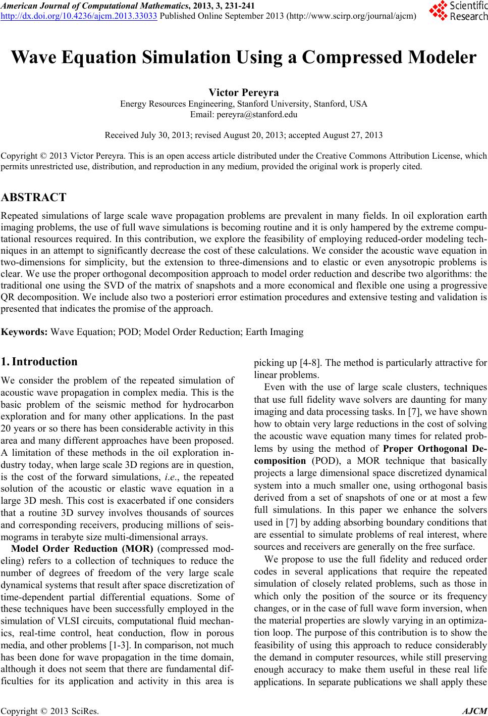
American Journal of Computational Mathematics, 2013, 3, 231-241
http://dx.doi.org/10.4236/ajcm.2013.33033 Published Online September 2013 (http://www.scirp.org/journal/ajcm)
Wave Equation Simulation Using a Compressed Modeler
Victor Pereyra
Energy Resources Engineering, Stanford University, Stanford, USA
Received July 30, 2013; revised August 20, 2013; accepted August 27, 2013
Copyright © 2013 Victor Pereyra. This is an open access article distributed under the Creative Commons Attribution License, which
permits unrestricted use, distribution, and reproduction in any medium, provided the original work is properly cited.
ABSTRACT
Repeated simulations of large scale wave propagation problems are prevalent in many fields. In oil exploration earth
imaging problems, the use of full wave simulations is becoming routine and it is only hampered by the extreme compu-
tational resources required. In this contribution, we explore the feasibility of employing reduced-order modeling tech-
niques in an attempt to significantly decrease the cost of these calculations. We consider the acoustic wave equation in
two-dimensions for simplicity, but the extension to three-dimensions and to elastic or even anysotropic problems is
clear. We use the proper orthogonal decomposition approach to model order reduction and describe two algorithms: the
traditional one using the SVD of the matrix of snapshots and a more economical and flexible one using a progressive
QR decomposition. We include also two a posteriori error estimation procedures and extensive testing and validation is
presented that indicates the promise of the approach.
Keywords: Wave Equation; POD; Model Order Reduction; Earth Imaging
1. Introduction
We consider the problem of the repeated simulation of
acoustic wave propagation in complex media. This is the
basic problem of the seismic method for hydrocarbon
exploration and for many other applications. In the past
20 years or so there has been considerable activity in this
area and many different approaches have been proposed.
A limitation of these methods in the oil exploration in-
dustry today, when large scale 3D regions are in question,
is the cost of the forward simulations, i.e., the repeated
solution of the acoustic or elastic wave equation in a
large 3D mesh. This cost is exacerbated if one considers
that a routine 3D survey involves thousands of sources
and corresponding receivers, producing millions of seis-
mograms in terabyte size multi-dimensional arrays.
Model Order Reduction (MOR) (compressed mod-
eling) refers to a collection of techniques to reduce the
number of degrees of freedom of the very large scale
dynamical systems that result after space discretization of
time-dependent partial differential equations. Some of
these techniques have been successfully employed in the
simulation of VLSI circuits, computational fluid mechan-
ics, real-time control, heat conduction, flow in porous
media, and other problems [1-3]. In comparison, not much
has been done for wave propagation in the time domain,
although it does not seem that there are fundamental dif-
ficulties for its application and activity in this area is
picking up [4-8]. The method is particularly attractive for
linear problems.
Even with the use of large scale clusters, techniques
that use full fidelity wave solvers are daunting for many
imaging and data processing tasks. In [7], we have shown
how to obtain very large reductions in the cost of solving
the acoustic wave equation many times for related prob-
lems by using the method of Proper Orthogonal De-
composition (POD), a MOR technique that basically
projects a large dimensional space discretized dynamical
system into a much smaller one, using orthogonal basis
derived from a set of snapshots of one or at most a few
full simulations. In this paper we enhance the solvers
used in [7] by adding absorbing boundary conditions that
are essential to simulate problems of real interest, where
sources and receivers are generally on the free surface.
We propose to use the full fidelity and reduced order
codes in several applications that require the repeated
simulation of closely related problems, such as those in
which only the position of the source or its frequency
changes, or in the case of full wave form inversion, when
the material properties are slowly varying in an optimiza-
tion loop. The purpose of this contribution is to show the
feasibility of using this approach to reduce considerably
the demand in computer resources, while still preserving
enough accuracy to make them useful in these real life
applications. In separate publications we shall apply these
C
opyright © 2013 SciRes. AJCM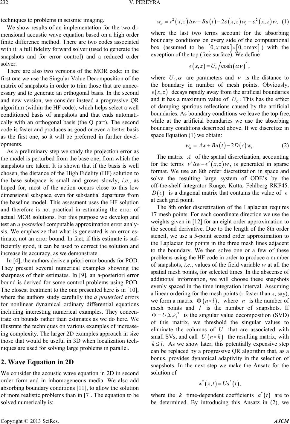

V. PEREYRA
232
techniques to problems in seismic imaging.
We show results of an implementation for the two di-
mensional acoustic wave equation based on a high order
finite difference method. There are two codes associated
with it: a full fidelity forward solver (used to generate the
snapshots and for error control) and a reduced order
solver.
There are also two versions of the MOR code: in the
first one we use the Singular Value Decomposition of the
matrix of snapshots in order to trim those that are unnec-
essary and to generate an orthogonal basis. In the second
and new version, we consider instead a progressive QR
algorithm (within the HF code), which helps select a well
conditioned basis of snapshots and that ends automati-
cally with an orthogonal basis (the Q part). The second
code is faster and produces as good or even a better basis
as the first one, so it will be preferred in further devel-
opments.
As a preliminary step we study the projection error as
the model is perturbed from the base one, from which the
snapshots are taken. It is shown that if the basis is well
chosen, the distance of the High Fidelity (HF) solution to
the base subspace is small and grows slowly, i.e., as
hoped for, most of the action occurs close to this low
dimensional subspace, even for substantial departures from
the baseline model. This assesment uses the HF solution
and therefore is not practical in estimating the error of
actual MOR solutions. For this purpose we develop and
test an a posteriori computable approximation error analy-
sis. We emphasize that what is generated is an error es-
timate, not an error bound. In fact, if this estimate is suf-
ficiently good, it can be used to correct the solution and
increase its accuracy, as we demonstrate.
In [4], the authors derive a priori error bounds for POD.
They present several numerical examples showing the
sharpness of their estimates. In [9], an a-posteriori error
bound is derived for some control problems using POD.
The closest treatment to the one presented here is in [10],
where the authors study carefully the a posteriori errors
for nonlinear dynamical ordinary differential equations
including interesting numerical examples. They concen-
trate on bounds rather than estimates as we do here. We
illustrate the techniques on various examples of increase-
ing complexity. The larger 2D examples approach in size
those that would be useful in 3D when localization tech-
niques are used for solving large problems in parallel.
2. Wave Equation in 2D
We consider the acoustic wave equation in 2D in second
order form and in inhomogeneous media. We also add
absorbing boundary conditions [11], to allow the solution
of more realistic problems than in [7]. The equation to be
solved numerically is:



 
22
,2,
tt t
wvxzwButxz wxz w   ,, (1)
where the last two terms account for the absorbing
boundary conditions on every side of the computational
box (assumed to be




0,max0, maxxz) with the
exception of the top (free surface). We define
 
2
0
,coshxzU  ,
where 0,U

are parameters and

is the distance to
the boundary in number of mesh points. Obviously,


,
x
z decays rapidly away from the artificial boundaries
and it has a maximum value of 0. This has the effect
of damping spurious reflections caused by the artificial
boundaries. As boundary conditions we leave the top free,
while at the artificial boundaries we use the absorbing
boundary conditions described above. If we discretize in
space Equation (1) we obtain:
U
 
2
tt t
wAwBut Dw . (2)
The matrix
A
of the spatial discretization, accounting
for the terms


22
,vw xzw, is generated in sparse
format. We use an 8th order discretization in space and
solve the resulting large system of ODE’s by the
off-the-shelf integrator Runge, Kutta, Fehlberg RKF45.


D is a diagonal matrix that contains the value of
at each grid point.

The 8th order discretization of the Laplacian requires
17 mesh points. For each coordinate direction we use the
weights given in [12] for an eight order approximation to
the second derivative. Due to the length of the 8th order
stencil, we use a 5-point second order approximation to
the Laplacian for points in the three mesh lines adjacent
to the boundary. We then solve one or a few of these
problems using the HF code in order to produce a number
of snapshots, i.e., values of the field variable w at all the
spatial mesh points, for selected times. In the abscense of
additional information, we will choose these snapshots
evenly spaced in the time integration interval. Assuming
a linear ordering for the mesh points (z faster than x, say),
we form a matrix


,nl

 where is the number of
mesh points and l is the number of snapshots. If
is the singular value decomposition (SVD)
of this matrix, we threshold the singular values to
eliminate the columns of U that are associated with
small SVs, and call
n
T
lll
UV 


Unk

the resulting matrix, with
.kl

As we show later, this potentially expensive step
can be replaced by a progressive QR algorithm that, as a
bonus, provides dynamical adaptivity in the selection of
snapshots. In the next step we make the Ansatz for the
solution of


**
,,wxt Uat

where the time-dependent coefficients k


*
at are to
be determined. By introducing this Ansatz in (2), we

V. PEREYRA 233
obtain a Galerkin projection method, resulting in a reduced
order model that approximates the original dynamical
system:


*T*T T
2.
tt t
aUAUaU ButU DUa*
In this step we have used that U is an orthogonal
matrix. Observe that this method can be extended to
three dimensions and to elastic or even anisotropic equa-
tions. The difficulty there will be the problem size and
complexity.
Implementation
We implement the above method in two separate codes
for simplicity.
1) HFWave is the High Fidelity solver that is capable
of running multiple problems, varying either the position
or the frequency of the source, or the velocity.
For each run a seismic section (i.e., a collection of
time histories at selected output points), and also a sepa-
rate time history, are output for comparison and verifica-
tion purposes.
2) MORWave solves the reduced problem, with the
same capabilities of running multiple problems as HFWave.
For each problem it outputs a seismic section and trace as
HFWave, for comparison and verification.
3. Numerical Examples of 2D Acoustic Wave
Propagation
3.1. Example 1
For the first comparison of the High Fidelity (HF) and
Reduced Order (MOR) solvers performance, we use a
simple model that consists of three flat layers with con-
stant velocities; see Table 1.
The other parameters for this run are:
#points in x-direction: 351
#points in z-direction: 351
dx = dy = 10; dt = 0.005
#snapshots: 400
alpha = 0.18
U0 = 200.
The source is a Hz Ricker wavelet placed at the
mesh point (x = 1600, z = 50). We collect time histories
at 101 equally spaced receivers starting at x = 700. Ob-
serve that is the snapshot time spacing. The Runge-
Kutta-Fehlberg ODE integrator RKF45 chooses its own
timestep dynamically to satisfy stability and accuracy
5
dt
Table 1. Model vel3l.
Depth (m) Velocity (m/sec)
0 - 1500 1000
1500 - 2500 2000
2500 - 3000 3000
requirements (for a 4 10

absolute and relative errors).
We run five shots starting at , spaced at 20 m.
400 equally spaced HF snapshots are used from the first
and last shot. The rank of the projection is 33.
1600x
Results are shown in Table 2. In Figure 1, we show
the cross-plots of the HF and MOR solutions for a shot at
the end point of the shot interval, while in Table 3 we list
the Residual Mean Squares for every shot. The RMS is
calculated over the whole section. We observe that the
errors, as expected, are smaller at the end shots and in-
crease towards the middle of the interval; also, even in
the worst case the phases are very accurate, with the
inacuracies concentrated in the amplitudes. This is a
good sign, since in most imaging tasks the phases (arrival
times) are more important than the amplitudes (only rela-
tive amplitudes of events are meaningful).
3.2. Example 2
For the second example we consider a problem similar to
the BP model of [7] that we call vel4pc. Instead of a fully
inhomogeneous velocity, as in that example, we have
binned the velocity and used an average velocity to obtain
a piecewise constant model that preserves most of the
geological complexity of the original one (see Figure 2).
Figure 1. Crossplot of one trace: HF vs MOR. Problem
vel3l.
Table 2. Results for model vel3l. 5 shots.
vel3l # Equations.#Timest. Pre-proc. Integ.
HF 246,402 8850 - 168.17”
MOR 66 4004 548.23” 4.0”
Ratio 3733 2.2 - 42.04”
Table 3. RMS for the various shots. Model vel3l.
Shot 1 2 3 4 5
RMS 0.03 0.2 0.23 0.14 0.03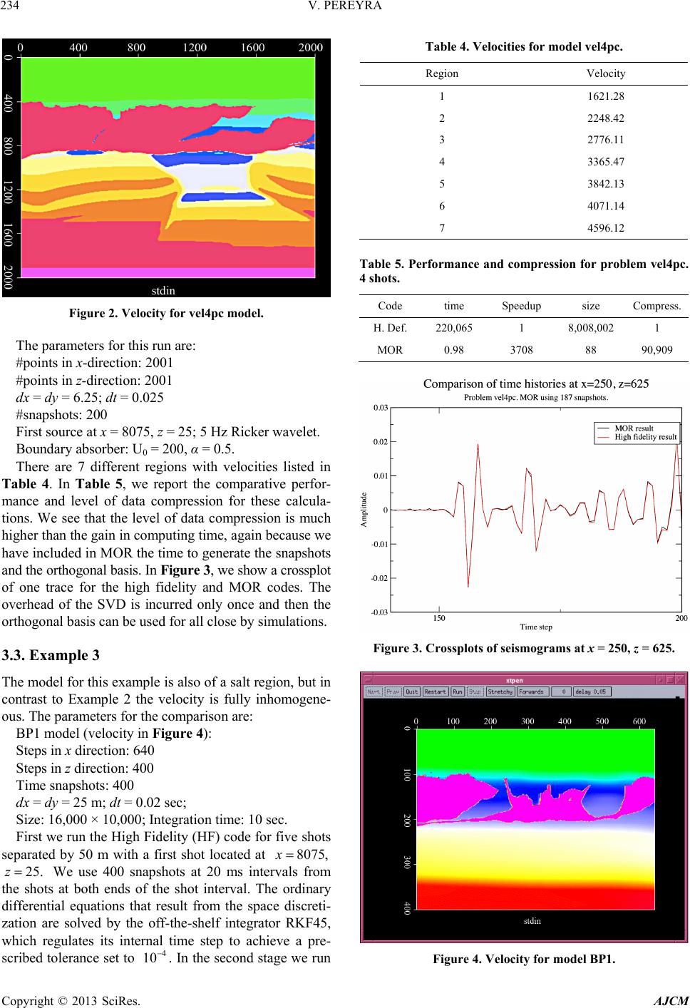

V. PEREYRA
234
Figure 2. Velocity for vel4pc model.
The parameters for this run are:
#points in x-direction: 2001
#points in z-direction: 2001
dx = dy = 6.25; dt = 0.025
#snapshots: 200
First source at x = 8075, z = 25; 5 Hz Ricker wavelet.
Boundary absorber: U0 = 200, α = 0.5.
There are 7 different regions with velocities listed in
Table 4. In Table 5, we report the comparative perfor-
mance and level of data compression for these calcula-
tions. We see that the level of data compression is much
higher than the gain in computing time, again because we
have included in MOR the time to generate the snapshots
and the orthogonal basis. In Figure 3, we show a crossplot
of one trace for the high fidelity and MOR codes. The
overhead of the SVD is incurred only once and then the
orthogonal basis can be used for all close by simulations.
3.3. Example 3
The model for this example is also of a salt region, but in
contrast to Example 2 the velocity is fully inhomogene-
ous. The parameters for the comparison are:
BP1 model (velocity in Figure 4):
Steps in x direction: 640
Steps in z direction: 400
Time snapshots: 400
dx = dy = 25 m; dt = 0.02 sec;
Size: 16,000 × 10,000; Integration time: 10 sec.
First we run the High Fidelity (HF) code for five shots
separated by 50 m with a first shot located at 8075,x

We use 400 snapshots at 20 ms intervals from
the shots at both ends of the shot interval. The ordinary
differential equations that result from the space discreti-
zation are solved by the off-the-shelf integrator RKF45,
which regulates its internal time step to achieve a pre-
scribed tolerance set to . In the second stage we run
25.z
4
10
Table 4. Velocities for model vel4pc.
Region Velocity
1 1621.28
2 2248.42
3 2776.11
4 3365.47
5 3842.13
6 4071.14
7 4596.12
Table 5. Performance and compression for problem vel4pc.
4 shots.
Code time Speedup size Compress.
H. Def. 220,065 1 8,008,002 1
MOR 0.98 3708 88 90,909
Figure 3. Crossplots of seismograms at x = 250, z = 625.
Figure 4. Velocity for model BP1.

V. PEREYRA 235
the Model Order Reduced code for the same five shots.
In both cases we produce one section with 360 receivers
spaced by 25 m, starting at 4975.x

The statistics are
given in Table 6.
In Figures 5-7, we show cross-plots of a trace at x =
4975 for HF and MOR, corresponding to three shots.
3.4. Example 4
For this example we consider the inhomogeneous version
of model BP (see Example 2) that we call vel4 (Figure 8.
i The size of the mesh is the same as before, but now we
have: dx = dy = 6.25 dt = 0.025 #snapshots: 400 Source
at x = 6250, z = 125; 5 Hz Ricker wavelet. The results are
shown in Figure 9 and Table 7.
4. Applications
The results of the previous section show that we can re-
produce accurately the solution of the wave equation
using projections on a small space of snapshots with
considerable savings in computing time. Reverse time
migration of seismic data [13] requires simulating the
Table 6. Results for model BP1.
BP1 # Equations. #Timest. Pre-process Total time
HF 514,082 23,746 - 1936.5
MOR 574 12,147 1826'' 16.6
Ratio 896 1.95 - 117
Table 7. Results for model vel4. 9 sources.
vel4 # Equations. #Timest. Pre-proc. Total time
HF 8,008,002 117,694 - 130,275”
MOR 726 13,087 14,908” 68.4”
Ratio 11,030 9 - 1904”
Figure 5. Crossplot for first shot. Model BP1. HF vs MOR.
Figure 6. Crossplot for shot 2.
Figure 7. Crossplot for shot 3.
Figure 8. Velocity model for vel4.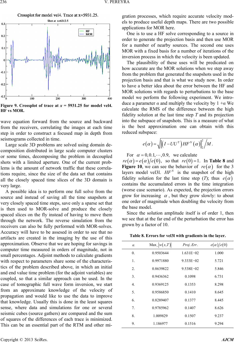

V. PEREYRA
236
Figure 9. Crossplot of trace at x = 5931.25 for model vel4.
HF vs MOR.
wave equation forward from the source and backward
from the receivers, correlating the images at each time
step in order to construct a focused map in depth from
seismograms collected in time.
Large scale 3D problems are solved using domain de-
composition distributed in large scale computer clusters
or some times, decomposing the problem in decoupled
shots with a limited aperture. One of the current prob-
lems is the amount of network traffic that these correla-
tions require, since the size of the data set that contains
all the closely spaced time slices of the 3D domain is
very large.
A possible idea is to perform one full solve from the
source and instead of saving all the time snapshots at
very closely spaced time steps, save only a sparse set that
is then used to MOR-solve and produce the closely
spaced slices on the fly instead of having to move them
through the network. The reverse simulation from the
receivers can also be fully performed with MOR-solves.
Accuracy will have to be assesed in order to see that no
artifacts are created in the imaging by the use of this
approximation. Observe that we are hoping for savings in
computer time measured in orders of magnitude, not in
small percentages. Adjoint methods to calculate gradients
with respect to parameters share some of the characteris-
tics of the problem described above, in which an initial
and end value time problem (for the adjoint variables) are
coupled, so that a similar approach can be used. In the
case of tomographic full wave form inversion, we start
from an approximate knowledge of the velocity of
propagation and would like to use the data to improve
that knowledge. Usually this is done in the least squares
sense, where data and simulations for one or several
seismic cubes (source gathers) are compared and the sum
of squares of the differences of each trace is minimized.
This can be an essential part of the RTM and other mi-
gration processes, which require accurate velocity mod-
els to produce useful depth maps. There are two possible
applications for MOR here.
One is to use a HF solve corresponding to a source in
order to generate the projection basis and then use MOR
for a number of nearby sources. The second one uses
MOR with a fixed basis for a number of iterations of the
inversion process in which the velocity is been updated.
The plausibility of these uses will be predicated on
how accurate are the MOR solutions when we step away
from the problem that generated the snapshots used in the
projection basis and that is what we study now. In order
to have a better idea about the error between the HF and
MOR solutions with regards to perturbations to the base
model we perform the following experiment. We intro-
duce a parameter α and multiply the velocity by 1 +α We
calculate the RMS of the difference between the high
fidelity solution at the last time step T and its projection
into the subspace of snapshots. This is a measure of what
is the best approximation one can obtain with this
reduced subspace:



2
T
2.
N
eIUUHF   M
For 0, 0.1,, 0.9,


 we calculate






0,ree e   so that In Table 8 and
Figure 10, we can see the behavior of

01re .

re

for the 3
layers model vel3l. N
H
F is the snapshot of the high
fidelity solution for the last time step (T); thus


e

contains the accumulated errors in the time integration
(worse case scenario). As expected, the projection errors
grow for increasing

, but they grow slowly: to about
one order of magnitude when doubling the velocity from
the base model.
Since the solution amplitude itself is of order 1, then
we see that at the far end of the perturbation the error has
grown by a factor of 10.
Table 8. Errors for vel3l with gradients in the layer.
α 
Max ,
xwxT ..Proj Err




0ee 
0. 0.9503644 1.631E−02 1.000
1. 0.9971880 9.333E−02 5.721
2. 0.8639822 9.538E−02 5.846
3. 0.9436362 0.1098 6.731
4. 0.9369125 0.1353 8.298
5. 0.9586850 0.1410 8.645
6. 0.8289407 0.1377 8.445
7. 0.9785962 0.1407 8.626
8. 1.009829 0.1507 9.237
9. 1.186977 0.1516 9.294

V. PEREYRA 237
Figure 10. Projection errors.
5. Global Error Estimation-I
In the previous section we demonstrated the behavior of
the error of MOR when perturbing the problem, using the
exact high fidelity solution to calculate it. Of course, in
practice, when we are solving a reduced problem for an
equation different from the base one that generated the
snapshots we will not have the HF solution. Thus, in this
section we use ideas of deferred corrections [14-16] to
produce a computable a posteriori error estimate that
does not require the HF solution.
In [17], a different procedure for estimating a post-
eriori the projection errors in a Krilov algorithm por a
nonlinear problem is described. Grepl and Patera [18]
consider a posteriori error bounds for parabolic equations
when using a reduced-basis method and they apply them
to construct a basis by a greedy algorithm.
We start from the HF equation
 
2
tt t
wAwBut Dw  (3)
and consider also the reduced one
 



 
11T111T1T11
2
tt t
aUAUaUButUDUa,
1.
T
1T
(4)
where stands for our initial selection of orthogonal
basis vectors.

1
U
For simplicity we assume that the discretization errors
are negligible compared to the approximation error, al-
though they can also be easily accounted for. Putting
and calling we get:
 
11
wUa

2t LA D 
  

 

11 111
11 1
,
,
tt
tt
UaP LUaBut
wPLwBut






(5)
where is the projector on the space
generated by the columns of . This equation tells us
that the whole trajectory stays in the subspace
  111
PUU

1
U


1
wt
spanned by We will also use the projector on the
orthogonal complement Now we
introduce

1.U
 
UU
  11
.PIUU


1
,V

21




 an orthogonal basis for a
larger subspace of snapshots (observe that
 
12
PU


1
0,V




 ). The easiest
way to do this is to select a good number of snapshots,
perform the SVD and then use a large threshold to
choose the first set of basis functions. In the second pass
one would lower the threshold and use the original and
additional basis functions as and so on.
 
1T 11T
VP UV


2
U
With this new basis, we obtain a more accurate ap-
proximation by solving the reduced equation
 

2T 2.
tt
bU LUbBut




 (6)
Then, by solving this small dimensional problem, we
obtain the corrected solution: and the ap-
proximation error for can be es-
timated by It is important to remark that
this is not a bound for the error, but it actually comes
with a sign and, if the procedure has been performed
appropriately, not only can be used to estimate the error
with high precision but, just as in the deferred correction
approach, should be more accurate than and
the process can be iterated by adding more basis func-
tions as required. If one starts with a lax threshold for the
singular values and proceeds with this algorithm by re-
fining the basis, then this is also a multi-resolution ap-
proach, in which one solves first for a low frequency
band and keeps adding frequencies as needed. On the
down side, the procedure will give a good estimate pro-
vided that is a sufficiently accurate proxy for the
HF solution.
  22
wU

1
w

1
w
b

tw  
 
21
.ww 

2
w

2
w

1
w
If both solutions are inaccurate, this approach can lead
to a significant under-estimation of the error.
6. Global Error Estimation-II
In this section we will pursue a different approach to
solve the error estimation problem. In the first step we
solve (4). We define , the
approximation to


 

 

11111
tUetVdt  


t


1.PBu t 

w

1,U

1
U
w

1
w
.w
,


that we wish to calculate. By
substracting (5) from (3) we get:
tt This is the exact error
equation, which shows the components in each subspace,
reflecting the fact that since the HF solution will not
usually belong to the space spanned by there will
certainly be an error component in the orthogonal com-
plement of that space. That there is also a component of
the error in the space of the columns of comes
from the fact that usually the projection of into that
space will not coincide with [10]. A problem with
this equation is that we do not know But if we re-
place it by

11
LwP Lw  

1
w


then this can be solved approxi-
mately for

1

in the reduced space

2:U

V. PEREYRA
238
 


11 ,
tt LPLw But



or
 


111 111.
tt tt
UeVdL PLwBut 


Multiplying the previous equation successively by
, a
, we get the coupled sys-
tem:

1
U
res
and nd calling


1
V

11
V





T1
wLwBu t
 
11T
,
tt
eUL


 

11T 1
.
tt
dVLresw  
Thus, we need now to pre-calculate:
and
We proceed in
stages. First we solve the reduced system with the initial
basis produ Then we use this to
obtain and solve the error system to
obtain and from them
  1T1,ULU
 1
a
 
11T 1
,,ULV V LU
 1
Ucin
 1,wres w
,ed
 
1T 1.VLV
 1.

1.
g a



1

 
7. A Progressive Algorithm
The developments of the previous sections suggest the
possibility of devising an incremental algorithm, in which
a solution for a given basis is updated when new vectors
are introduced in the basis.
Using the notation above we consider not the error
equation but rather the solution of the reduced equation
with an enlarged basis: Replacing
this Ansatz in the wave equation we get:
 
21 1
.wUaVb
 
11 1.
tttt
UaVbLUaBu LVb 
1
1
1
Replacing we get:
  1,Ua w
 




11 111
.
tt tt
wVbPLw BuPLw BuLVb

 
The first terms on both sides cancel out and we are left
with an equation on the subspace spanned by the col-
umns of :

1
V
 

1T11 .
tt
bVLVbresw (7)
Observe that this is the same as the second equation
for the error if we set the component Thus, we
first solve for in the the space spanned by the
columns of U and then we can add a correction to
that solution by solving Equation (7) for
0.e

1:b

1
w
 1

1
V
 
21 .wU b

1
a
8. Numerical Test
We test first the direct procedure with the problem for
model vel3l described in Section 3, Example 1. We run
the HF code and MOR with SV thresholds 0.01, 0.005
This leads to basis with 57 and 64 snapshots, respectively.
The results are shown in Figures 11 and 12, with the
Figure 11. HF vs two MOR runs with different thresholds
for first shot.
Figure 12. Exact and estimated errors for first shot.
estimated error tracking closely the exact one (including
its sign!).
Now we test the second procedure on the same prob-
lem, selecting for MOR a threshold of 0.05 that results in
45 snapshots been selected. For the extended space we
choose the same threshold as above. Results can be seen
in Figures 13-16. We see that both procedures give very
good results.
9. Adaptive Snapshot Selection
An interesting and novel approach to a dynamic selection
of snapshots can be achieved by using a progressive QR
decomposition [19]. This will also eliminate the need for
the SVD of the snapshot’s matrix. The strategy is as
follows:
 Within the HF integration process, as a snapshot is
produced, calculate one step of the QR reduction via a
Householder transformation. If the diagonal term in R
is below a given threshold, reject it, otherwise accept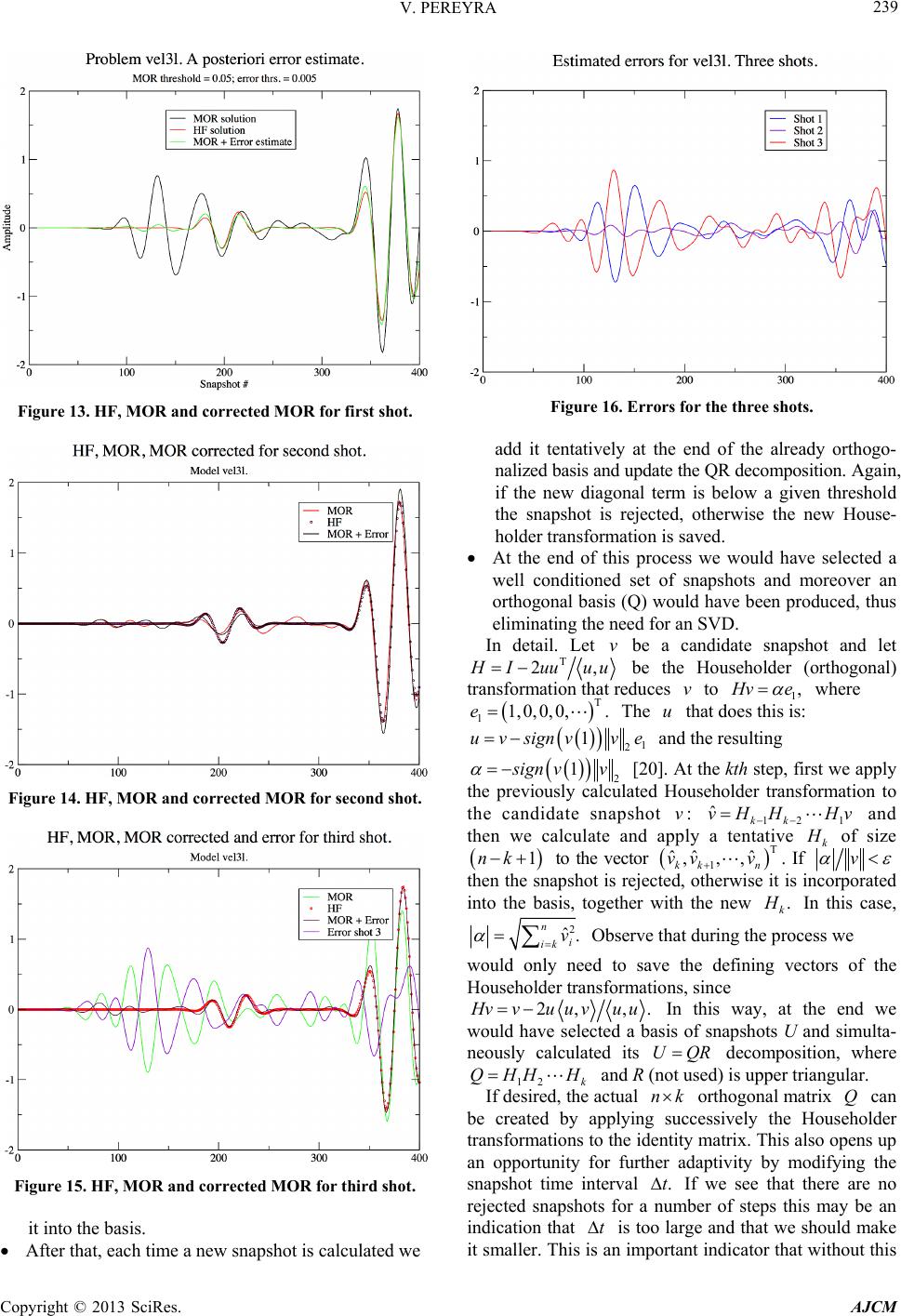

V. PEREYRA 239
Figure 13. HF, MOR and corrected MOR for first shot.
Figure 14. HF, MOR and corrected MOR for second shot.
Figure 15. HF, MOR and corrected MOR for third shot.
it into the basis.
 After that, each time a new snapshot is calculated we
Figure 16. Errors for the three shots.
add it tentatively at the end of the already orthogo-
nalized basis and update the QR decomposition. Again,
if the new diagonal term is below a given threshold
the snapshot is rejected, otherwise the new House-
holder transformation is saved.
 At the end of this process we would have selected a
well conditioned set of snapshots and moreover an
orthogonal basis (Q) would have been produced, thus
eliminating the need for an SVD.
In detail. Let
v
be a candidate snapshot and let
T
2
H
,Iuu uu be the Householder (orthogonal)
transformation that reduces to 1 v,
H
ve

 where
The u that does this is:

T
11,0,0,0, .e




1
2
1uvsignv ve and the resulting




2
1
s
ign vv   [20]. At the kth step, first we apply
the previously calculated Householder transformation to
the candidate snapshot :
v
12 1 and
then we calculate and apply a tentative
ˆkk
vHH Hv


k
H
of size


1nk

 to the vector kkn . If

T
1ˆ
,,,v

ˆˆ
vv v



then the snapshot is rejected, otherwise it is incorporated
into the basis, together with the new .
k
H
In this case,
2
ˆ.
n
i
ik
v 

 Observe that during the process we
would only need to save the defining vectors of the
Householder transformations, since
2, ,.
H
vvuuv uu In this way, at the end we
would have selected a basis of snapshots U and simulta-
neously calculated its UQR

decomposition, where
12 k
QHHH

 and R (not used) is upper triangular.
If desired, the actual nk

orthogonal matrix can
be created by applying successively the Householder
transformations to the identity matrix. This also opens up
an opportunity for further adaptivity by modifying the
snapshot time interval
Q
.t

If we see that there are no
rejected snapshots for a number of steps this may be an
indication that t

is too large and that we should make
it smaller. This is an important indicator that without this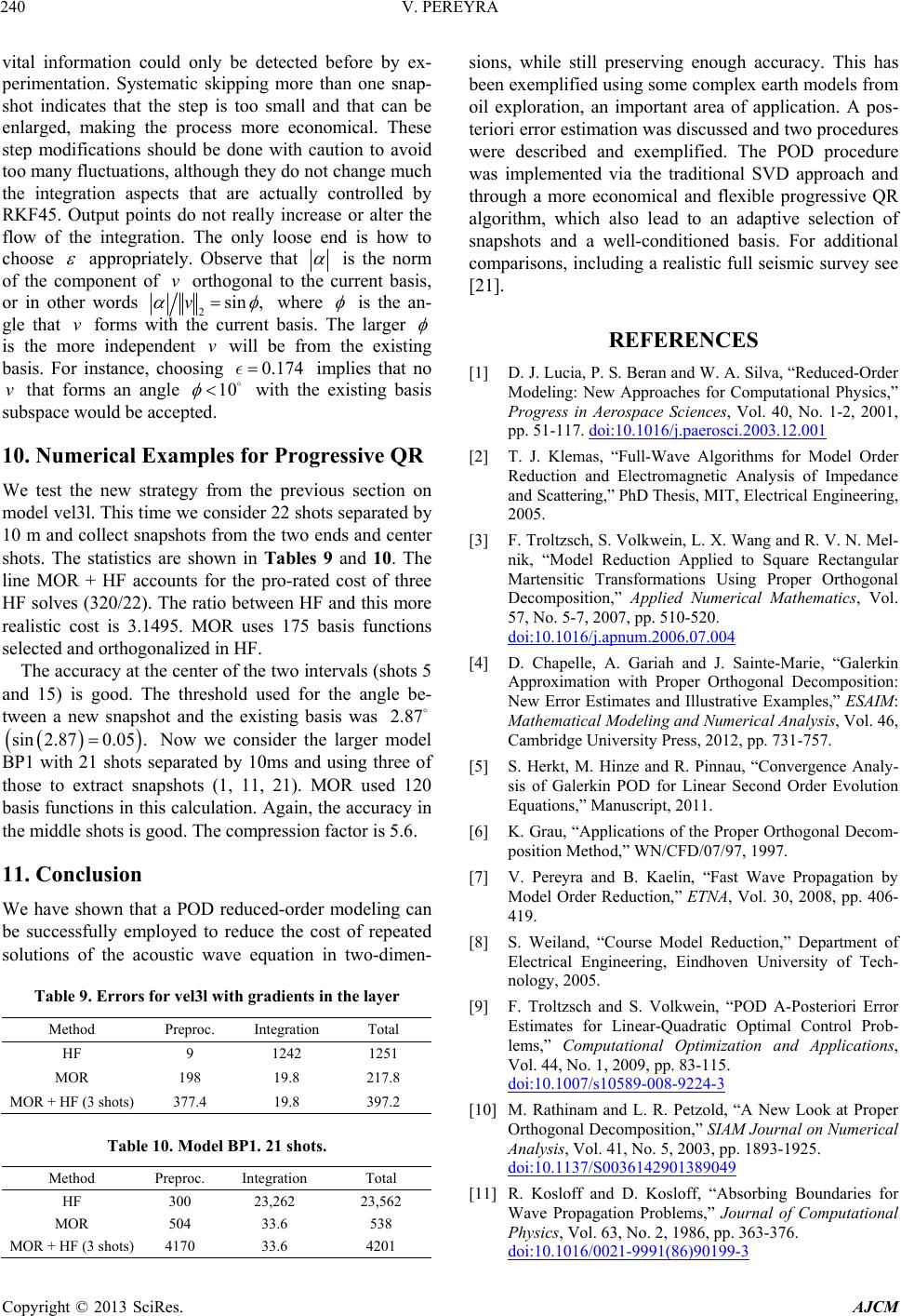

V. PEREYRA
240
vital information could only be detected before by ex-
perimentation. Systematic skipping more than one snap-
shot indicates that the step is too small and that can be
enlarged, making the process more economical. These
step modifications should be done with caution to avoid
too many fluctuations, although they do not change much
the integration aspects that are actually controlled by
RKF45. Output points do not really increase or alter the
flow of the integration. The only loose end is how to
choose

appropriately. Observe that

is the norm
of the component of
v
orthogonal to the current basis,
or in other words 2sin ,v

  where

is the an-
gle that forms with the current basis. The larger v

is the more independent will be from the existing
basis. For instance, choosing implies that no
v
0.174
v
that forms an angle 10



 with the existing basis
subspace would be accepted.
10. Numerical Examples for Progressive QR
We test the new strategy from the previous section on
model vel3l. This time we consider 22 shots separated by
10 m and collect snapshots from the two ends and center
shots. The statistics are shown in Tables 9 and 10. The
line MOR + HF accounts for the pro-rated cost of three
HF solves (320/22). The ratio between HF and this more
realistic cost is 3.1495. MOR uses 175 basis functions
selected and orthogonalized in HF.
The accuracy at the center of the two intervals (shots 5
and 15) is good. The threshold used for the angle be-
tween a new snapshot and the existing basis was
Now we consider the larger model
BP1 with 21 shots separated by 10ms and using three of
those to extract snapshots (1, 11, 21). MOR used 120
basis functions in this calculation. Again, the accuracy in
the middle shots is good. The compression factor is 5.6.
2.87



.87sin20.05 .
11. Conclusion
We have shown that a POD reduced-order modeling can
be successfully employed to reduce the cost of repeated
solutions of the acoustic wave equation in two-dimen-
Table 9. Errors for vel3l with gradients in the layer
Method Preproc. Integration Total
HF 9 1242 1251
MOR 198 19.8 217.8
MOR + HF (3 shots) 377.4 19.8 397.2
Table 10. Model BP1. 21 shots.
Method Preproc. Integration Total
HF 300 23,262 23,562
MOR 504 33.6 538
MOR + HF (3 shots) 4170 33.6 4201
sions, while still preserving enough accuracy. This has
been exemplified using some complex earth models from
oil exploration, an important area of application. A pos-
teriori error estimation was discussed and two procedures
were described and exemplified. The POD procedure
was implemented via the traditional SVD approach and
through a more economical and flexible progressive QR
algorithm, which also lead to an adaptive selection of
snapshots and a well-conditioned basis. For additional
comparisons, including a realistic full seismic survey see
[21].
REFERENCES
[1] D. J. Lucia, P. S. Beran and W. A. Silva, “Reduced-Order
Modeling: New Approaches for Computational Physics,”
Progress in Aerospace Sciences, Vol. 40, No. 1-2, 2001,
pp. 51-117. doi:10.1016/j.paerosci.2003.12.001
[2] T. J. Klemas, “Full-Wave Algorithms for Model Order
Reduction and Electromagnetic Analysis of Impedance
and Scattering,” PhD Thesis, MIT, Electrical Engineering,
2005.
[3] F. Troltzsch, S. Volkwein, L. X. Wang and R. V. N. Mel-
nik, “Model Reduction Applied to Square Rectangular
Martensitic Transformations Using Proper Orthogonal
Decomposition,” Applied Numerical Mathematics, Vol.
57, No. 5-7, 2007, pp. 510-520.
doi:10.1016/j.apnum.2006.07.004
[4] D. Chapelle, A. Gariah and J. Sainte-Marie, “Galerkin
Approximation with Proper Orthogonal Decomposition:
New Error Estimates and Illustrative Examples,” ESAIM:
Mathematical Modeling and Numerical Analysis, Vol. 46,
Cambridge University Press, 2012, pp. 731-757.
[5] S. Herkt, M. Hinze and R. Pinnau, “Convergence Analy-
sis of Galerkin POD for Linear Second Order Evolution
Equations,” Manuscript, 2011.
[6] K. Grau, “Applications of the Proper Orthogonal Decom-
position Method,” WN/CFD/07/97, 1997.
[7] V. Pereyra and B. Kaelin, “Fast Wave Propagation by
Model Order Reduction,” ETNA, Vol. 30, 2008, pp. 406-
419.
[8] S. Weiland, “Course Model Reduction,” Department of
Electrical Engineering, Eindhoven University of Tech-
nology, 2005.
[9] F. Troltzsch and S. Volkwein, “POD A-Posteriori Error
Estimates for Linear-Quadratic Optimal Control Prob-
lems,” Computational Optimization and Applications,
Vol. 44, No. 1, 2009, pp. 83-115.
doi:10.1007/s10589-008-9224-3
[10] M. Rathinam and L. R. Petzold, “A New Look at Proper
Orthogonal Decomposition,” SIAM Journal on Numerical
Analysis, Vol. 41, No. 5, 2003, pp. 1893-1925.
doi:10.1137/S0036142901389049
[11] R. Kosloff and D. Kosloff, “Absorbing Boundaries for
Wave Propagation Problems,” Journal of Computational
Physics, Vol. 63, No. 2, 1986, pp. 363-376.
doi:10.1016/0021-9991(86)90199-3

V. PEREYRA
241
[12] H. B. Keller and V. Pereyra, “Symbolic Generation of
Finite Difference Formulas,” Mathematics of Computa-
tion, Vol. 32, 1978, pp. 955-971.
doi:10.1090/S0025-5718-1978-0494848-1
[13] B. Biondi and G. J. Shan, “Prestack Imaging of Over-
turned Reflections by Reverse Time Migration,” SEG
Annual Meeting, 2002.
[14] V. Pereyra, “Iterated Deferred Corrections for Nonlinear
Operator Equations,” Numerische Mathematik, Vol. 10,
No. 4, 1967, pp. 316-323. doi:10.1007/BF02162030
[15] V. Pereyra, J. W. Daniel and L. L. Schumaker, “Iterated
Deferred Corrections for Initial Value Problems,” Acta
Científica Venezolana, Vol. 19, 1968, pp. 128-135.
[16] P. E. Zadunaisky, “A Method for the Estimation of Errors
Propagated in the Numerical Solution of a System of Or-
dinary Differential Equations,” In: G. I. Kontopoulos, Ed.,
The Theory of Orbits in the Solar System and in Stellar
Systems. Proceedings from Symposium No. 25 Held in
Thessaloniki, International Astronomical Union, Acade-
mic Press, London, 1964, p. 281.
[17] M. Rewienski and J. White, “A Trajectory Piecewise-
Linear Approach to Model Order Reduction and Fast
Simulation of Nonlinear Circuits and Micromachined
Devices,” IEEE Transactions on Computer-Aided Design
of Integrated Circuits and Systems, Vol. 22, No. 2, 2003,
pp. 155-170. doi:10.1109/TCAD.2002.806601
[18] M. A. Grepl and A. T. Patera, “A Posteriori Error Bounds
for Reduced-Basis Approximations of Parametrized Para-
bolic Partial Differential Equations,” ESAIM: Mathe-
matical Modelling and Numerical Analysis, Vol. 39, No.
1, 2005, pp. 157-181. doi:10.1051/m2an:2005006
[19] G. H. Golub and C. F. Van Loan, “Matrix Computations,”
3rd Edition, Johns Hopkins University Press, Baltimore,
1996.
[20] P. C. Hansen, V. Pereyra and G. Scherer, “Least Squares
Data Fitting with Applications,” Johns Hopkins Univer-
sity Press, Baltimore, 2012.
[21] C. L. Wu, D. Bevc and V. Pereyra, “Model Order Reduc-
tion for Efficient Seismic Modeling,” Accepted for Pub-
lication in SEG 83rd Annual Meeting Extended Abstracts,
Houston, 2013.