Paper Menu >>
Journal Menu >>
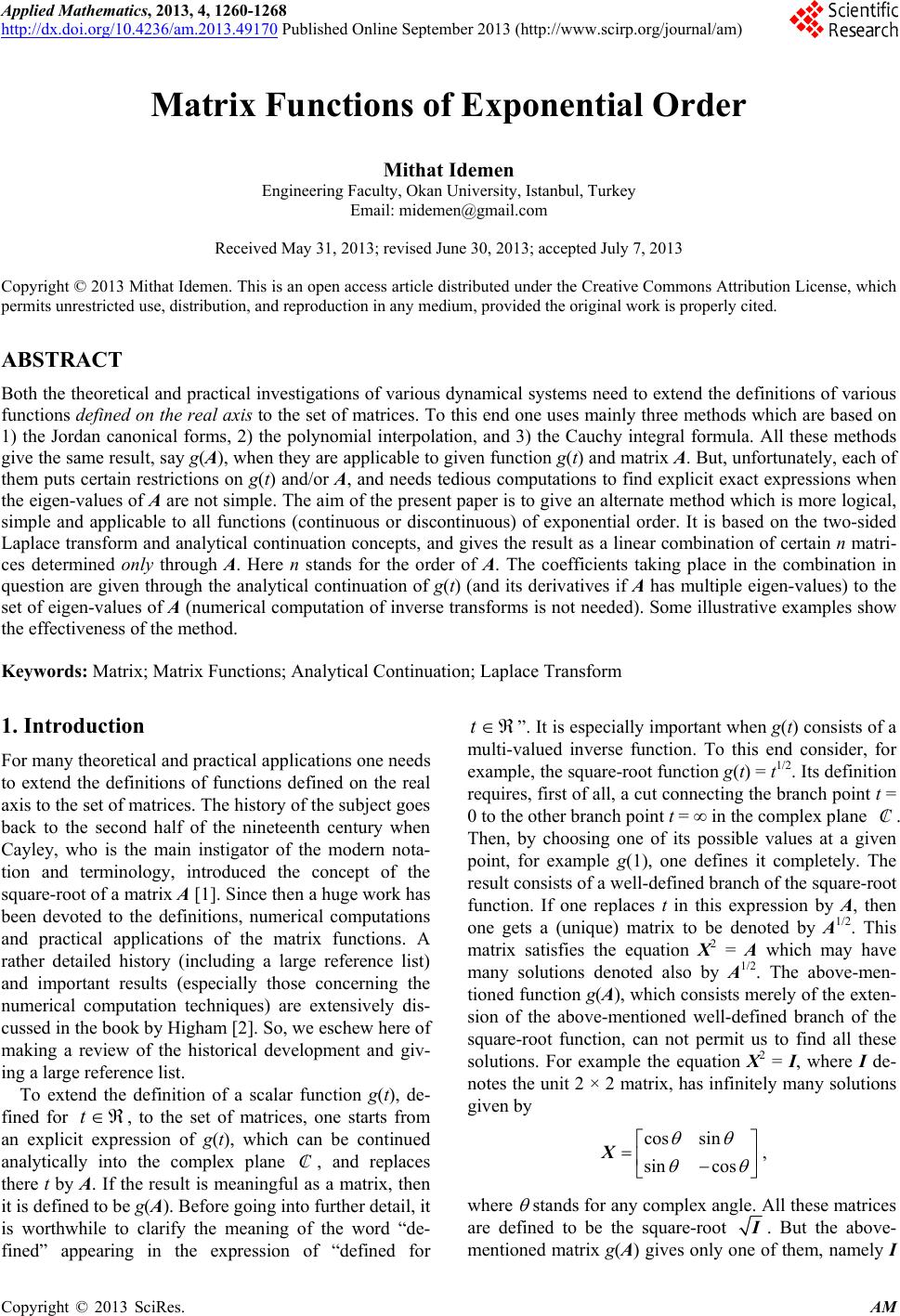 Applied Mathematics, 2013, 4, 1260-1268 http://dx.doi.org/10.4236/am.2013.49170 Published Online September 2013 (http://www.scirp.org/journal/am) Matrix Functions of Exponential Order Mithat Idemen Engineering Faculty, Okan University, Istanbul, Turkey Email: midemen@gmail.com Received May 31, 2013; revised June 30, 2013; accepted July 7, 2013 Copyright © 2013 Mithat Idemen. This is an open access article distributed under the Creative Commons Attribution License, which permits unrestricted use, distribution, and reproduction in any medium, provided the original work is properly cited. ABSTRACT Both the theoretical and practical investigations of various dynamical systems need to extend the definitions of various functions defined on the real axis to the set of matrices. To this end one uses mainly three methods which are based on 1) the Jordan canonical forms, 2) the polynomial interpolation, and 3) the Cauchy integral formula. All these methods give the same result, say g(A), when they are applicable to given function g(t) and matrix A. But, unfortunately, each of them puts certain restrictions on g(t) and/or A, and needs tedious computations to find explicit exact expressions when the eigen-values of A are not simple. The aim of the present paper is to give an alternate method which is more logical, simple and applicable to all functions (continuous or discontinuous) of exponential order. It is based on the two-sided Laplace transform and analytical continuation concepts, and gives the result as a linear combination of certain n matri- ces determined only through A. Here n stands for the order of A. The coefficients taking place in the combination in question are given through the analytical continuation of g(t) (and its derivatives if A has multiple eigen-values) to the set of eigen-values of A (numerical computation of inverse transforms is not needed). Some illustrative examples show the effectiveness of the method. Keywords: Matrix; Matrix Functions; Analytical Continuation; Laplace Transform 1. Introduction For many theoretical and practical applications one needs to extend the definitions of functions defined on the real axis to the set of matrices. The history of the subject goes back to the second half of the nineteenth century when Cayley, who is the main instigator of the modern nota- tion and terminology, introduced the concept of the square-root of a matrix A [1]. Since then a huge work has been devoted to the definitions, numerical computations and practical applications of the matrix functions. A rather detailed history (including a large reference list) and important results (especially those concerning the numerical computation techniques) are extensively dis- cussed in the book by Higham [2]. So, we eschew here of making a review of the historical development and giv- ing a large reference list. To extend the definition of a scalar function g(t), de- fined for , to the set of matrices, one starts from an explicit expression of g(t), which can be continued analytically into the complex plane C, and replaces there t by A. If the result is meaningful as a matrix, then it is defined to be g(A). Before going into further detail, it is worthwhile to clarify the meaning of the word “de- fined” appearing in the expression of “defined for t t Th ”. It is especially important when g(t) consists of a multi-valued inverse function. To this end consider, for example, the square-root function g(t) = t1/2. Its definition requires, first of all, a cut connecting the branch point t = 0 to the other branch point t = in the complex plane C. en, by choosing one of its possible values at a given point, for example g(1), one defines it completely. The result consists of a well-defined branch of the square-root function. If one replaces t in this expression by A, then one gets a (unique) matrix to be denoted by A1/2. This matrix satisfies the equation X2 = A which may have many solutions denoted also by A1/2. The above-men- tioned function g(A), which consists merely of the exten- sion of the above-mentioned well-defined branch of the square-root function, can not permit us to find all these solutions. For example the equation X2 = I, where I de- notes the unit 2 × 2 matrix, has infinitely many solutions given by cos sin sin cos X, where stands for any complex angle. All these matrices are defined to be the square-root I. But the above- mentioned matrix g(A) gives only one of them, namely I C opyright © 2013 SciRes. AM 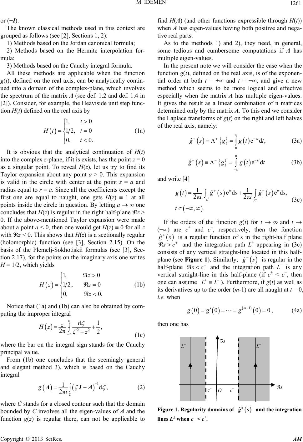 M. IDEMEN 1261 or (−I). The known classical methods used in this context are grouped as follows (see [2], Sections 1, 2): 1) Methods based on the Jordan canonical formula; 2) Methods based on the Hermite interpolation for- mula; 3) Methods based on the Cauchy integral formula. All these methods are applicable when the function g(t), defined on the real axis, can be analytically contin- ued into a domain of the complex-plane, which involves the spectrum of the matrix A (see def. 1.2 and def. 1.4 in [2]). Consider, for example, the Heaviside unit step func- tion H(t) defined on the real axis by 1, 0 12, 0 0, 0. t Ht t t (1a) It is obvious that the analytical continuation of H(t) into the complex z-plane, if it is exists, has the point z = 0 as a singular point. To reveal H(z), let us try to find its Taylor expansion about any point a > 0. This expansion is valid in the circle with center at the point z = a and radius equal to r = a. Since all the coefficients except the first one are equal to naught, one gets H(z) 1 at all points inside the circle in question. By letting a one concludes that H(z) is regular in the right half-plane z > 0. If the above-mentioned Taylor expansion were made about a point a < 0, then one would get H(z) 0 for all z with z < 0. This shows that H(z) is a sectionally regular (holomorphic) function (see [3], Section 2.15). On the basis of the Plemelj-Sokhotiskii formulas (see [3], Sec- tion 2.17), for the points on the imaginary axis one writes H = 1/2, which yields 1, 0 12, 0 0, 0 z Hz z z. (1b) Notice that (1a) and (1b) can also be obtained by com- puting the improper integral 22 1 d, 2π2 z Hz z (1c) where the bar on the integral sign stands for the Cauchy principal value. From (1b) one concludes that the seemingly general and elegant method 3), which is based on the Cauchy integral 1 1d, 2πC gi AIA (2) where C stands for a closed contour such that the domain bounded by C involves all the eigen-values of A and the function g(z) is regular there, can not be applicable to find H(A) (and other functions expressible through H(t)) when A has eigen-values having both positive and nega- tive real parts. As to the methods 1) and 2), they need, in general, some tedious and cumbersome computations if A has multiple eigen-values. In the present note we will consider the case when the function g(t), defined on the real axis, is of the exponen- tial order at both t = + and t = −, and give a new method which seems to be more logical and effective especially when the matrix A has multiple eigen-values. It gives the result as a linear combination of n matrices determined only by the matrix A. To this end we consider the Laplace transforms of g(t) on the right and left halves of the real axis, namely: 0 ˆed, st g sggt t (3a) 0 ˆed st g sggt t (3b) and write [4] 11 ˆˆ eded, 2π2π ,. ts ts LL g tgssgs ii t s (3c) If the orders of the function g(t) for t and t (−) are c+ and c−, respectively, then the function ˆ g s is a regular function of s in the right-half plane s c and the integration path L+ appearing in (3c) consists of any vertical straight-line located in this half- plane (see Figure 1). Similarly, ˆ g s is regular in the half-plane s c L and the integration path L− is any vertical straight-line in this half-plane (if c+ < c−, then one can assume L ). Furthermore, if g(t) as well as its derivatives up to the order (m-1) are all naught at t = 0, i.e. when 1 00 0 m gg g 0 , (4a) then one has c − O c + s s L + L − Figure 1. Regularity domains of ˆ g s and the integration lines L when c− < c+. Copyright © 2013 SciRes. AM 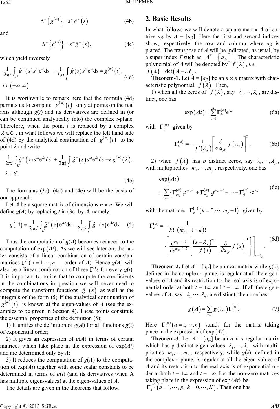 M. IDEMEN 1262 ˆ mm g sg s (4b) and ˆ, mm g sg s (4c) which yield inversely 11 ˆˆ ed ed, 2π2π ,. m mts mts LL g ss sgss sgt ii t (4d) It is worthwhile to remark here that the formula (4d) permits us to compute m g t only at points on the real axis although g(t) and its derivatives are defined in (or can be continued analytically into) the complex t-plane. Therefore, when the point t is replaced by a complex C , in what follows we will replace the left hand side of (4d) by the analytical continuation of m g t to the point and write 11 ˆˆ ed ed, 2π2π . m ms ms LL gsss gsssg ii C (4e) The formulas (3c), (4d) and (4e) will be the basis of our approach. Let A be a square matrix of dimensions n n. We will define g(A) by replacing t in (3c) by A, namely: 11 ˆˆ edsed. 2π2π ss LL g gsgs s ii AA A (5) Thus the computation of g(A) becomes reduced to the computation of exp{At}. As we will see later on, the lat- ter consists of a linear combination of certain constant matrices j ( = order of A). Hence g(A) will also be a linear combination of these j’s for every g(t). It is important to notice that to compute the coefficients in the combinations in question we will never need to compute the transform functions 1, ,jn ˆ g s as well as the integrals of the form (5) if the analytical continuation of m g t is known at the eigen-values of A (see the ex- amples to be given in Section 4). These points constitute the essential properties of the definition (5): 1) It unifies the definition of g(A) for all functions g(t) of exponential order; 2) It gives an expression of g(A) in terms of certain matrices which take place in the expression of exp(At) and are determined only by A; 3) It reduces the computation of g(A) to the computa- tion of exp(At) together with some scalar constants to be determined in terms of g(t) (and its derivatives when A has multiple eigen-values) at the eigen-values of A. The details are given in the theorems that follow. 2. Basic Results In what follows we will denote a square matrix A of en- tries ajk by A = [ajk]. Here the first and second indices show, respectively, the row and column where ajk is placed. The transpose of A will be indicated, as usual, by a super index T such as . The characteristic polynomial of A will be denoted by T T jk a A f , i.e. detf A I. Theorem-1. Let A = [ajk] be an n n matrix with char- acteristic polynomial f . Then, 1) when all the zeros of f , say 1,, n , are dis- tinct, one has 0 1 expeα nλt α t ΓA (6a) with 0 Γ given by T 0 1, jk f a f Γ (6b) 2) when f has p distinct zeros, say 1,, p , with multiplicities 1,, p mm, respectively, one has 12 12 0 1 exp e p mm mm t tt t A (6c) with the matrices 0, ,1 k km a Γ given by T 1 1 1 ! 1! d. d k m mk mk jk s km k sfs a fs s Γ (6d) Theorem-2. Let A = [ajk] be an nn matrix while g(z), defined in the complex z-plane, is regular at all the eigen- values of A and its restriction to the real axis is of expo- nential order at both t = + and t = −. If all the eigen- values of A, say 1,, n , are distinct, then one has 0 1 . n gg ΓA (7) Here stands for the matrix taking place in the expression of exp{At}. 0 1,,a Γ n Theorem-3. Let A = [ajk] be an n n regular matrix which has p distinct eigen-values 1,, p with multi- plicities 1,, p mm 1,,; 0ap , respectively, while g(z), defined in the complex z-plane, is regular at all the eigen-values of A and its restriction to the real axis is of exponential or- der at both t = + and t = −. Let the non-zero matrices taking place in the expression of exp{At} be . Then one has , ,k ΓK k C opyright © 2013 SciRes. AM 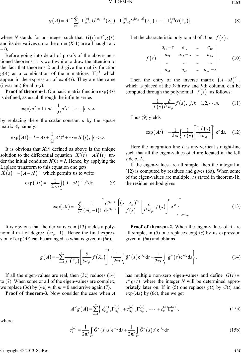 M. IDEMEN Copyright © 2013 SciRes. AM 1263 G 12 12 0 1 , pmm N mm gGG ΓΓ ΓAA (8) where N stands for an integer such that N Gtt gt and its derivatives up to the order (K-1) are all naught at t = 0. Let the characteristic polynomial of A be f s: 11 121 21 222 12 ... ... ...... ... ... ... n n nn nn as aa aasa fs aaa Before going into detail of proofs of the above-men- tioned theorems, it is worthwhile to draw the attention to the fact that theorems 2 and 3 give the matrix function g(A) as a combination of the n matrices k Γ which appear in the expression of exp(At). They are the same (invariant) for all g(t). s . (10) Then the entry of the inverse matrix 1 s AI, which is placed at the k-th row and j-th column, can be computed through the polynomial f s as follows: Proof of theorem-1. Our basic matrix function exp{At} is defined, as usual, through the infinite series 1, ,1,2,,. jk f sjk n a fs (11) 22 1 exp1, 2! atatatt Thus (9) yields by replacing there the scalar constant a by the square matrix A, namely: T 11 exped. 2π ts jk L fs ts i a fs A (12) 22 1 exp, . 2! tI tttt AAA X Here the integration line L is any vertical straight-line such that all the eigen-values of A are located in the left side of L. It is obvious that X(t) defined as above is the unique solution to the differential equation tXX'A t un- der the initial condition X(0) = I. Hence, by applying the Laplace transform to this equation one gets 1 ˆ– ss X AI which permits us to write 1ts 1 exped. 2πL tss i AAI If the eigen-values are all simple, then the integral in (12) is computed by residues and gives (6a). When some of the eigen-values are multiple, as stated in theorem-1b, the residue method gives (9) T 1 1 1 . 1d exp e 1! d m m p st m jk s s tf a mfs s s A (13) Proof of theorem-2. When the eigen-values of A are all simple, in (5) one replaces exp(As) by its expression given in (6a) and obtains It is obvious that the derivatives in (13) yields a poly- nomial in t of degree . Hence the final expres- sion of exp(At) can be arranged as what is given in (6c). 1m T 1 111 ˆˆ ed ed 2π2π ns jk LL s g fgss gs fa ii s A. (14) If all the eigen-values are real, then (3c) reduces (14) to (7). When some or all of the eigen-values are complex, we replace (3c) by (4e) with m = 0 and arrive again (7). Proof of theorem-3. Now consider the case when A has multiple non-zero eigen-values and define Gt N tgt where the integer N will be determined appro- priately later on. If in (5) one replaces g(t) by G(t) and exp{As} by (6c), then we get 112 200 1 , p N mmm m gcc c ΓΓ ΓAA (15a) where 11 ˆˆ de e 2π2π ss kk k LL cGsssGss ii ds (15b) 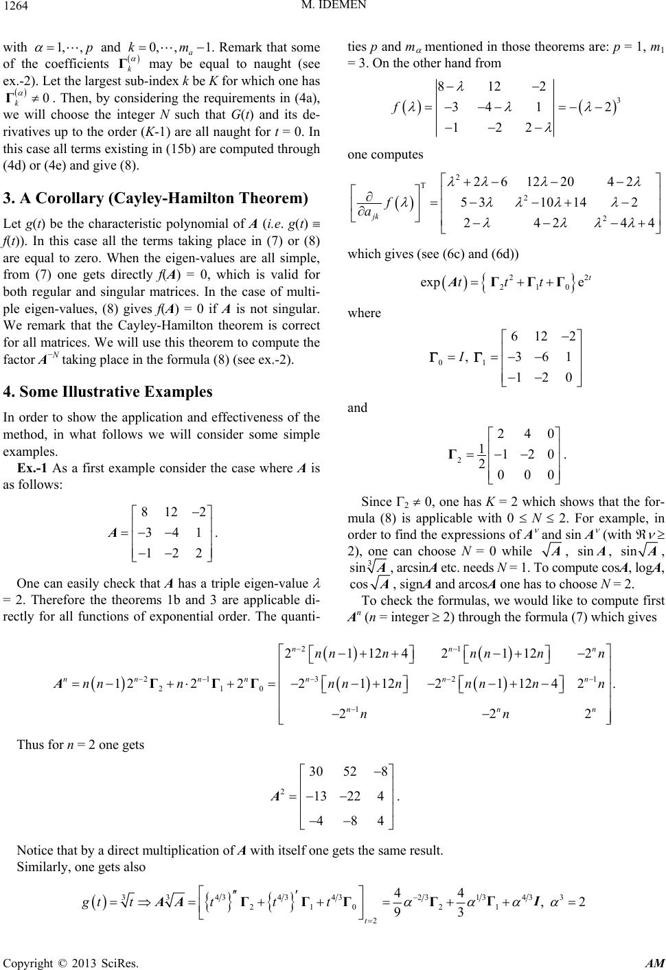 M. IDEMEN 1264 with 1,,p e coeffici and . Remark that some hents 0, ,1 a km k of t Γ may be equal ub-index k be K nsi to naught (see vativ Let g(t) be the characteristic polynomial of A (i.e. g(t) ) In order to show the application and effectiveness of the ider some simple One can easily check that A has a tple eigen-value = 2. Therefore the theorems 1b and 3 are applicable di- re ties p and m mention = 3. On the other hand ex.-2)rgest s for which one has 0 k Γ. Then, by codering the requirements in (4a), we will choose the integer N such that G(t) and its de- ries up to the order (K-1) are all naught for t = 0. In this case all terms existing in (15b) are computed through (4d) or (4e) and give (8). 3. A Corollary (Cayley-Hamilton Theorem) . Let the la f(t)). In this case all the terms taking place in (7) or (8 are equal to zero. When the eigen-values are all simple, from (7) one gets directly f(A) = 0, which is valid for both regular and singular matrices. In the case of multi- ple eigen-values, (8) gives f(A) = 0 if A is not singular. We remark that the Cayley-Hamilton theorem is correct for all matrices. We will use this theorem to compute the factor A−N taking place in the formula (8) (see ex.-2). 4. Some Illustrative Examples method, in what follows we will cons examples. Ex.-1 As a first example consider the case where A is as follows: 812 2 341 122 A. ri ctly for all functions of exponential order. The quanti- ed in those theorems are: p = 1, m1 from 3 8122 34f 1 2 122 one computes T f 2 2 2 2612204 2 5 310142 24244 jk a which gives (see (6c) and (6d)) 22 10 exp et tttΓΓΓA 2 where 01 612 2 , 361 120 I and 2 240 1120 2000 Γ. Since 2 0, one has K = 2 which ows that the for- mula (8) is applicable with 0 N 2. For example, in or sh der to find the expressions of A and sin A (with 2), one can choose N = 0 while A, sin A, sin A, 3 sin A, arcsinA etc. needs N = 1. To compute cosA, logA, cos A, signA and arcosA one has to choose N = 2. To check the formulas, we would like to compute first integer 2) through the formula (7) which gives An (n = 1 112421122 nn nnn nn 21 3 2 210 1 12 22211221 1242. 22 nn nnnnn nn nn nnn nnn nn nn 2 2 n nn 1 2 n ΓΓΓA Thus for n = 2 one gets 2 30 528 13224 484 A. Notice that by a direct multiplication of A with itself one gets the sam result. Similarly, one gets also e 4343 4323 3 34 tt t ΓΓΓ ΓAA 1343 3 210 21 2 4, 2 93 t ΓI gt t C opyright © 2013 SciRes. AM 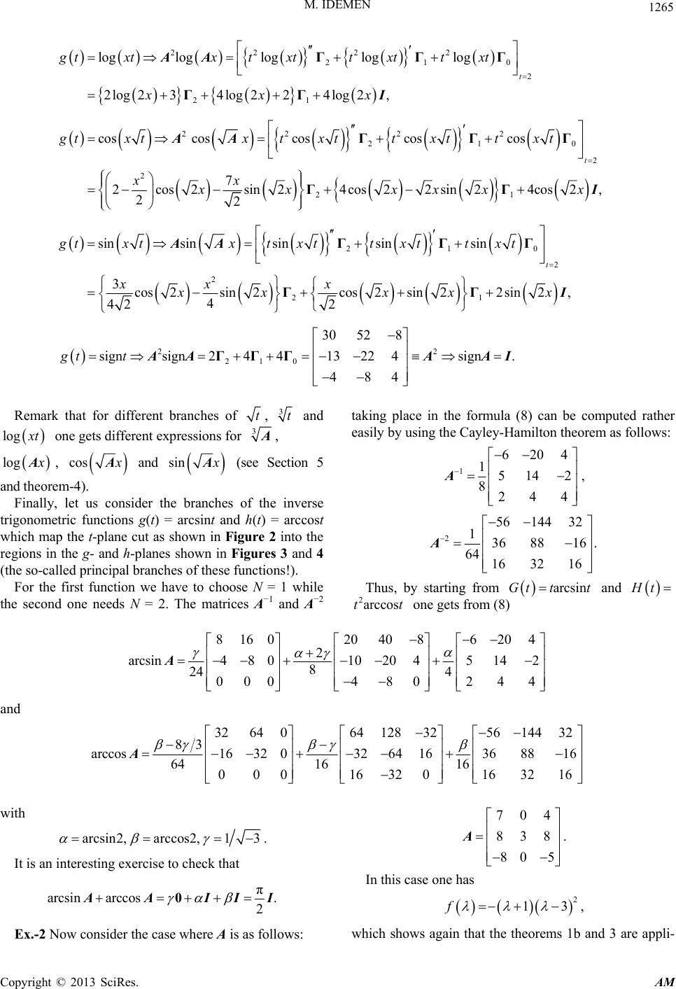 M. IDEMEN 1265 2222 21 2 21 log loglogloglog 2log234log224log2, t gtxtxt xtt xtt xt xxx ΓΓ ΓΓ AA I 0 Γ 22 22 21 2 2 21 cos cos coscoscos 7 2cos 2sin 24cos22sin 24cos2, 22 t gtxtxt xtt xtt xt xx 0 x xxxx x ΓΓ ΓΓ AA I Γ 21 2 2 21 sinsin sinsinsin 3cos2sin 2cos2sin22sin 2, 4 42 2 t gtxtxt xttxtt xt xx x xx xx ΓΓΓ ΓΓ AA I 0 x 2 2 210 30 528 signsign24413224sign. 484 gt t ΓΓΓ A AA AI Remark that for different branches of t, 3t and lo one gets different expressions for 3Ag x t , glo x A , cos x A and sin x A (sSection 5 ee and theo Finallylet us conse branche trigonome arcsint and ut as shown in Figure 2 into the re taking place in the formula (8) can be computed rather easily by using the Cayley-Hamilton theorem as follows: rem-4). , ider ths of the inverse tric functions g(t) = h(t) = arccost which map the t-plane c gions in the g- and h-planes shown in Figures 3 and 4 (the so-called principal branches of these functions!). For the first function we have to choose N = 1 while the second one needs N = 2. The matrices A−1 and A−2 1 6204 1514 2 8 244 A, 2 56144 32 1368816 . 64 1632 16 A Thus, by starting fromd arcsinGt tt an H t 2arccostt one gets from (8) 816 0 2 arcsin4 8 20 4 010 202 8 24 4 0004802 44 4086 20 45 14 A and 3264 064 1283256144 32 83 arccos16 32032 6416368816 6416 16 0001632 0163216 A with arcsin2,arccos2, 1 3 . an interesting exercise to check that It is π arcsin arccos . 2 0 A AIII 704 838 80 5 A. In this case one has which shows again that the theorems 1b and 3 are appli- Ex.-2 Now consider the case where A is as follows: 13f , 2 C opyright © 2013 SciRes. AM 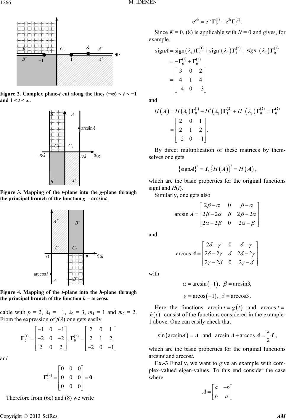 M. IDEMEN 1266 −1 1 B + B − C 2 A + A − C 1 t Figure 2. Complex plane-t cut along the lines (−) < t < −1 and 1 < t < . g B − C 2 C 1 A − −/2 /2 A + B + arcsin Figure 3. Mapping of the t-plane into the g-plane through the principal branch of the function g = arcsint. A − A + C 1 C 2 O h B + B − arccos Figure 4. Mapping of the t-plane into the h-plane through the principal branch of the function h = arccost. cable with p = 2, 1 = −1, 2 = 3, m1 = 1 and m2 = 2. From the expression of f( ) one gets easily Therefore from (6c) and (8) we write . Since K = 0, (8) is applicable with N = 0 and ges, for example, 2 Γ and 12 00 1012 0 1 202,212 ΓΓ 20220 1 and 2 1 000 000 Γ0. 000 12 3 00 ee e tt t ΓΓ A iv 12 10 2120 12 00 signsign 302 414 sign ΓΓ ΓΓ A sign 40 3 12 22 1021200 HH HH AΓΓ ΓΓ 201 212. 20 1 By direct multiplication of these matrices by them- selves one gets are the basic properties for the original functions signt and H(t). Similarly, one gets also 2 2 sign, HHAI AA, which 20 arcsin2 222 22 02 A and 20 arccos2222 22 02 A with arcsin1 ,arcsin3, arcos1 ,arccos3 . Here the functions and arcsin tgtarccos t ht consist of the functions considered k that in the e ove. One can easily chec xample- 1 ab and π arcsin arccos 2 AA, sin arcsin A AI h are the basic properties for the original functions t and arccost. Ex.-3 Finally, we want to give an exame with com- plex-valued eigen-values. To this end consider the case where whic arcsin pl ab ba A C opyright © 2013 SciRes. AM 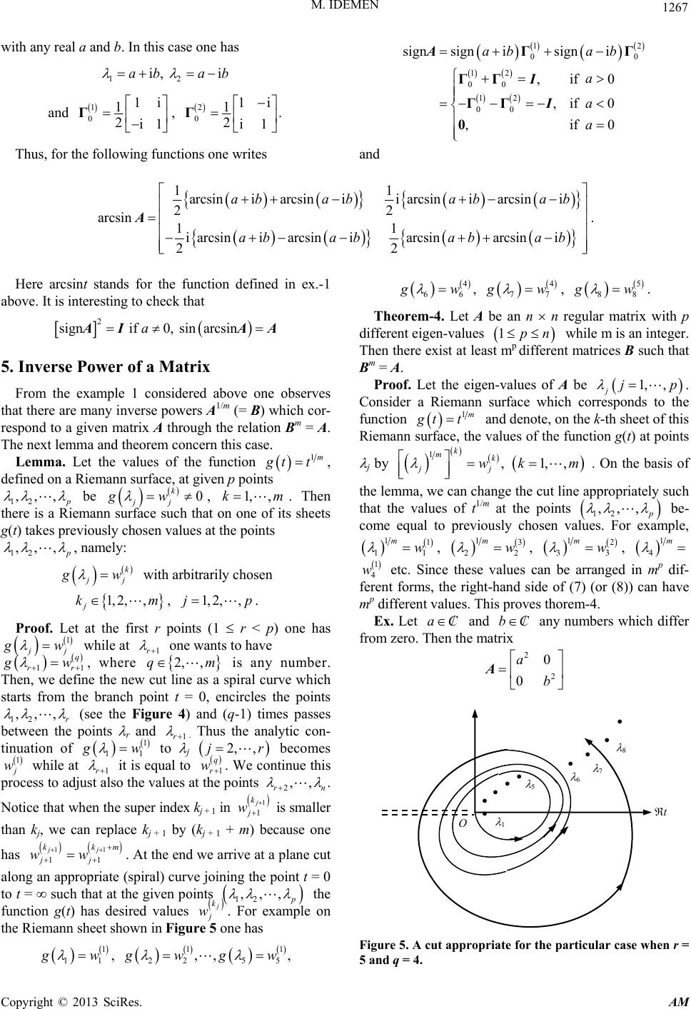 M. IDEMEN Copyright © 2013 SciRes. AM 1267 has with any real a and b. In this case one 12 00 12 00 12 00 sign signisigni if 0 ,if 0 ab ab a a ΓΓ ΓΓ ΓΓ A I 12 iabi,ab , I and 1 0 1i 1 2i1 Γ, 2 0 1i 1. 2i1 Γ ,i f 0a 0 and Thus, for the following functions one writes 11 arcsiniarcsinii arcsiniarcsini 22 arcsin 11 iarcsin iarcsin iarcsinarcsin i 2 2 ab abab ab ab abab ab A. Here arcsint stands for the function defined in ex.-1 above. It is interesting to check that A . Inverse Power of a Matrix m (= B) which cor- respond to a given matrix A through the relationm = A. The next lemma and theorem concern this case. nction 4 66 g w , 4 77 g w , 5 88 g w . Theorem-4. Let A be an n n regu matrix with p different eigen-values lar 2 sign if 0, sinarcsina AIA 1pn p different while m is an integer. Then there exist at least m matrices B such that Bm = A. co 5 Proof. Let the eigen-values of A be 1, , Consider a Riemann surface which the function jjp . rresponds to From the example 1 considered above one observes that there are many inverse powers A1/ 1m g tt and denote, one k-th sheet of this Riemann surface, the values of the function g(t) at th j by Bpoints 1, 1,, k mk jj wk m 1m g tt, Lemma. Let the values of the fu . On the basis of the lemma, we can ange the cut line appropriately such that the values of tm at the points defined on a Riemann surface, at given p points 12 ,,, p be 0 k jj gw , 1, ,km. Then there is a Riemann surface such that on one of its sheets g(t) takes previously chosen values at the points 1 ,,, ch 1/ ,,, 12 p be- co me equal to previously chosen values. For example, 2 p , namely: k j j g w with arbitrarily chosen j k2 Proof. Let at the first r points (1 r < p) o 1, 2,,, m1,,,j. p ne has 1 j j g w while at 1r one wants to have 11rr q g w , where ber. ne the ne which e branch pocirc 2, ,qm int t = 0, en is any num w cut line as a spiral curve les the points Then, we defi starts from th ,,, 12 r (see betw the Fi q-1) times passes gure 4) and ( een the points r and 1r . Thus the analytic con- tinuation of 1 11 g w to j 2, ,jr b ecomes 1 j w while at 1r it is e1r. We continue this process to adjust also the values at the points 2,, rn qual to q w . Nowhen the super index kj + 1 in 1 1 tice that j k j w is smaller than kj, we can replace kj + 1 (kj + 1 + m) because one has 1 11 j k jj ww . At the end at a plane cut along an appropriate (spiral) curve joining the oint 0 to t = such that at the given points ,, by mwe arrive pt = 1j k 12 , p the function g(t) has desired values j k j w. xample on For e the Riemann sheet shown in Figure 5 one has 1 11 g w , 11 22 55 ,, , g wg w 11 11 mw , 13 22 mw , 12 33 mw , 1 4 m 1 4 w etc. Since these valun be arranged in mp dif- fe es ca r (8)) can hav rent forms, the right-hand side of (7) (oe mp different values. This proves thorem-4. Ex. LetaC and bC any numbers which differ from zero. Then the matrix 2 2 0 0 a b A 1 7 6 5 O t 8 Figure 5. A cut appropriate for the particular case when r = 5 and q = 4.  M. IDEMEN 1268 has four square-roots given as follows: 0 b REFERENCES [1] A. Cayley, “A Memoir on the Theory of Matrices,” Phi- losophical Transactions of the Royal Society of London Vol. 148, 1858, pp. 17-37. doi:10.1098/rstl.1858.0002 00 0 , , , 00 0 0 aaa a bbb . , [2] N. J. Higham, “Functions of Matrices: Theory - putation,” Society for Industrial and Applied Mathe- matica (SIAM), Philadelphia, 2008. [3] N. I. Mushkhral Equations,” P. and Com elishvili, “Singular Integ Noordhoff Ltd., Holland, 1958. [4] E. C. Titchmarsh, “Introduction to the Theory of Fourier Integrals,” Chelsea Publishing Company, 1986, Chapter 1.3. C opyright © 2013 SciRes. AM |