Open Journal of Statistics, 2013, 3, 41-54
http://dx.doi.org/10.4236/ojs.2013.34A005 Published Online August 2013 (http://www.scirp.org/journal/ojs)
On the Use of Local Assessments for Monitoring Centrally
Reviewed Endpoints with Missing Data in Clinical Trials*
Sean S. Brummel1, Daniel L. Gillen2
1Harvard School of Public Health, Center for Biostatistics in AIDS Research, Boston, USA
2Department of Statistics, University of California, Irvine, USA
Received June 25, 2013; revised July 25, 2013; accepted August 2, 2013
Copyright © 2013 Sean S. Brummel, Daniel L. Gillen. This is an open access article distributed under the Creative Commons Attri-
bution License, which permits unrestricted use, distribution, and reproduction in any medium, provided the original work is properly
cited.
ABSTRACT
Due to ethical and logistical concerns it is common for data monitoring committees to periodically monitor accruing
clinical trial data to assess the safety, and possibly efficacy, of a new experimental treatment. When formalized, moni-
toring is typically implemented using group sequential methods. In some cases regulatory agencies have required that
primary trial analyses should be based solely on the judgment of an independent review committee (IRC). The IRC as-
sessments can produce difficulties for trial monitoring given the time lag typically associated with receiving assess-
ments from the IRC. This results in a missing data problem wherein a surrogate measure of response may provide use-
ful information for interim decisions and future monitoring strategies. In this paper, we present statistical tools that are
helpful for monitoring a group sequential clinical trial with missing IRC data. We illustrate the proposed methodology
in the case of binary endpoints under various missingness mechanisms including missing completely at random assess-
ments and when missingness depends on the IRC’s measurement.
Keywords: Group Sequential; Information; Independent Review; Endpoint; Missing Data
1. Introduction
When conducting a clinical trial that utilizes a subclinical
and/or subjective primary endpoint it may be necessary
to verify the local investigator assignment of the outcome
variable. Sometimes this verification is mandated by a
regulatory agency or it may be preferred by a study
sponsor. The advantage to verify the outcome is that it
may decrease misclassification of the outcome in studies
performed at multiple sites. As a recent example, consid-
er a phase II clinical trial to investigate the efficacy of an
experimental monoclonal antibody in combination with
chemotherapy in patients with relapsed chronic lympho-
cytic leukemia (CLL). A common endpoint in trials tar-
geting CLL is a binary indicator of complete response
(CR) of disease following the completion of the thera-
peutic regime. To standardize the assessment of CR in
CLL trials, most studies now use the NCI revised guide-
lines for determining CR [1], as shown in Figure 1. It is
clear that the CR criteria in Figure 1 are subclinical and
subjective in nature, requiring radiographic assessment of
lymph node size. In this case, the trial’s primary endpoint
may be validated by an independent review committee
(IRC). A recent a paper by Dodd et al. [2] reports an ad-
ditional seven trials that used an IRC to review the can-
cer progression measurements of a local investigator: two
renal cell carcinoma studies, one colorectal cancer study,
and four breast cancer studies.
In the setting of the CLL trial described above, it
would not be unusual for an independent data monitoring
committee (IDMC) to periodically assess the futility, and
possible efficacy, of the experimental intervention
through formal hypothesis testing. In this case a group
sequential framework would be natural for maintaining
frequentist error rates after conducting multiple interim
analyses of accruing data. A great deal of research has
been conducted in the area of group sequential methods
and it is well known that the operating characteristics of
a group sequential design depend on, among other things,
the exact timing of interim analyses. The timing of se-
quential analyses is measured by the proportion of statis-
tical information obtained at an interim analysis relative
to the maximal information that is anticipated at the final
analysis of the trial [3]. Thus it is important to reliably
*This research was supported in part by grant P30CA062203 from the
N
ational Cancer Institute (D.L.G.).
C
opyright © 2013 SciRes. OJS

S. S. BRUMMEL, D. L. GILLEN
42
Criteria for determining complete response (CR)
 Absence of lymphadenopathy, as confirmed by physical
examination and CT scan (i.e., all lymph nodes < 1.5 cm in
diameter).
 No hepatomegaly or splenomegaly, as confirmed by physical
examination and CT scan.
 Absence of B symptoms.
 Normal CBC as exhibited by
○ Polymorphonuclear leukocytes ≥ 1.5 × 109/L (without
granulocyte colony stimulating factor [GCSF] or other
colony stimulating factor support)
○ Platelets > 100 × 109//L (untransfused) or Hemoglobin
> 11.0 g/dL (untransfused and without erythropoietin or
othercolony stimulating factor support) or Lymphocyte
count ≤ 4 × 109/L
 Bone marrow biopsy indicating that bone marrow is
normocellular for age with less than 30% of the cells being
lymphocytes and lymphoid nodules absent.
Figure 1. Required criteria for determining a complete re-
sponse (CR) in chronic lymphocytic leukemia (CLL).
estimate statistical information at each interim analysis in
order to properly implement and potentially re-power a
chosen group sequential design [4,5]. However, when an
IRC is used to adjudicate a trial endpoint there may be a
subset of individuals who do not have verified IRC mea-
surements at the time of an interim analysis because the
final assessment of their outcome has yet to be re- turned
by the IRC. This results in a portion of trial pa- tients
whose primary response from the IRC is missing but
whose assessment from the local site (which is typi- cally
much quicker to obtain) is known. Relying solely upon
validated responses at the time of an interim analy- sis
can result in misleading estimates of statistical infor-
mation (at best) and opens the possibility of biased esti-
mates of treatment effect (at worst) [2,6]. While the local
investigator measurements only serve as a surrogate for
the IRC outcome measurements, use of this information
on observations that are missing validated outcomes may
be helpful in estimating statistical information for sam-
ple-size recalculations (also known as sample size re-
estimation) and for timing future analyses.
In the current manuscript we consider the use of in-
formation from local assessments when monitoring an
IRC validated binary endpoint such as that encountered
in the CLL trial described above. This setting allows us
to assess the proposed utility of local assessments in es-
timating statistical information in clinical trials where a
mean-variance relationship exists, and serves as a case
study for the importance of information estimation when
monitoring a clinical trial with group sequential stopping
boundaries. In Section 2 we discuss the importance of
accurately estimating statistical information when im-
plementing group sequential stopping rules. This section
concludes with an example to illustrate the impact that
missing IRC data can have on the operating characteris-
tics of a group sequential design. In Section 3, we pro-
pose missing data techniques to aid in estimating statis-
tical information and show how these methods can be
used for implementing group sequential tests. In Section
4 we present a simulation study to illustrate the utility of
the proposed approach and conclude with a discussion of
the challenges of monitoring group sequential clinical
trials with IRC validated endpoints.
2. The Role of Statistical Information in
Implementing Group Sequential Trial
Designs
Consider the CLL trial where interest lies in estimating
the effect of intervention on the probability of CR (a bi-
nary endpoint). Further, suppose that the ratio of the odds
of CR comparing intervention to control is used to assess
efficacy. Let ki denote the response of individual i in
treatment arm k (k = 1 for control, for interven-
tion) with associated response probabilities given by
Y
2k


PrpY1
ikk

. The odds of CR for group k is then
given by


1
kk k
Odds pp, , and the log-
odds ratio is given by
1, 2k

log Odds  2 Odds 1 . Finally,
suppose that the null hypothesis to be tested is 0:0H


against the one-sided alternative :0
a
H

.
Now consider a group sequential test of the above hy-
pothesis. For testing a one-sided alternative, many com-
monly used group sequential stopping rules consider
continuation sets of the form

,
j
jj
Cab

 such that
jj
ab

  for 1, ,jJ

 analyses. These bounda-
ries may be interpreted as the critical values for a deci-
sion rule. For instance, in the CLL trial a test statistic less
than
j
a would correspond to a decision in favor of su-
periority of the intervention while a test statistic exceed-
ing
j
b would correspond to a decision of futility re-
garding the intervention. Particular families of group
sequential designs correspond to parameterized boundary
functions that relate the stopping boundaries at succes-
sive analyses according to the proportion of statistical
information accrued. For instance, in the context of the
CLL trial, if we calculate a normalized statistic
ˆˆ Var
j
j
Z  j 



 where ˆ
j

is the maximum like-
lihood estimate of the log-odds ratio computed at analy-
sis j with corresponding variance ˆ
Var
j



, the propor-
tion of statistical information accrued at analysis j can be
calculated as


ˆˆ
Var Var
j
Jj




 where ˆ Var
j





is the variance of the maximum likelihood estimate of the
log-odds ratio computed at the final analysis of the trial
under a presumed maximal sample size. That is,
j

represents the fraction of total statistical information,
defined as the inverse of the variance of the final odds
ratio estimate, available from all patients at the time of
interim analysis j. It then follows that for some specified
parametric functions


*
f

, the critical values for a de-
cision rule at analysiscan be given by j


j
aj
af



S. S. BRUMMEL, D. L. GILLEN 43
and

j
bj
bf. For critical values on the normalized
Z-statistic scale, popular examples of

*
f
 include a
one-sided version of the Pocock [7] stopping rule that
takes

aj
f
G

, and a one-sided ver-
sion of the O’Brien-Fleming [8] stopping rule that takes

bj
f
12
aj j
fG

 , , where in both cases
the value of G is chosen to maintain a pre-specified type
I error rate.

bj
f
The choice of a stopping rule is generally based upon
the assessment of a wide range of statistical operating
characteristics across multiple candidate designs [3]. In
addition to type I error, commonly considered frequentist
operating characteristics include power, stopping prob-
abilities at each analysis, and average sample size. These
characteristics depend on the sampling distribution of the
test statistic under a given group sequential sampling
design. Unlike a fixed sample design where a single hy-
pothesis test is performed after the accrual of all trial data,
the sampling density of a test statistic in a group sequen-
tial framework not only depends upon the total amount of
statistical information accrued over the entire trial but
also on the timing of interim analyses as measured by the
proportion of the trial’s maximal statistical information,
j
, attained at each interim analysis [3]. Because of this,
there are usually at least two complicating factors that
must be dealt with during the monitoring of a clinical
trial. First, the schedule of interim analyses may not fol-
low the schedule assumed during the design of the trial.
Often, meetings of an IDMC are scheduled according to
calendar time, and thus the sample size available for
analysis at any given meeting is a random variable. Si-
milarly, accrual may be slower or faster than planned,
thereby resulting in a different number of interim analy-
ses than was originally planned. Because the exact stop-
ping boundaries are dependent upon the number and
timing of analyses, either of these scenarios will necessi-
tate modifications of the stopping rule. Second, the esti-
mate for response variability that was assumed at the
design phase is typically incorrect. As the trial progresses,
more accurate estimates may be obtained using available
data at each interim analysis. In this case, if one wishes
to maintain the originally specified power of the trial
then updates to the maximal sample size may be neces-
sary due to changes in variance estimates. Of course,
changes in maximal sample size will result in changes to
the proportion of information at all previously conducted
analyses.
Two ways to adjust for deviations in the timing of
planned analyses in order to maintain some of the trial’s
original operating characteristics include the error spend-
ing approach [9] and the constrained boundaries algo-
rithm [5]. First and foremost, these methods are primarily
used to maintain the size of the trial (type I error). A
choice must then be made as to whether the maximal
sample size or the power to detect a clinically relevant
alternative should be maintained. Briefly, the constrained
boundaries algorithm for maintaining the power of a
one-sided group sequential hypothesis test is imple-
mented as follows: At the design stage, boundary shape
functions are specified as and , where

aj
f
 
bj
f
j

denotes the planned proportion of maximal statisti-
cal information attained at interim analysis j, 1, ,jJ

,
with 1
J

. At the first analysis 1 is determined,
and stopping boundaries 1 and are computed. A
schedule of future analyses, 2

1
a b
,,
J
, which may dif-
fer from the originally assumed schedule of analyses is
then assumed and a stopping rule using the design para-
metric family


*
f

(constraining the first boundaries to
be 1 and 1) is found which has the desired power.
This consists of searching for a new maximal sample size
that has the correct type I error and power to detect the
alternative for the parametric design family for the as-
sumed schedule of interim analyses. At later analyses,
the exact stopping boundaries used at previously con-
ducted interim analyses are used as exact constraints at
those analysis times, and the stopping boundaries at the
current and all future analyses as well as the new maxi-
mal sample size needed to maintain statistical power are
re-computed using the parametric family of designs spe-
cified at the design stage and an assumed schedule of
future analysis times. Reference [5] notes that when
a b


aj
f

and


b
fj

are defined on the type I and II
error spending scales, this procedure is equivalent to the
error spending approach given in reference [10].
As noted above, in cases where power is to be main-
tained the current best estimate of the variance of the
response variable at each interim analysis is typically
used in place of the variance assumed at the design stage.
Use of a more accurate estimate of the response variabil-
ity, and hence statistical information, at earlier analyses
provides more accurate estimates of the maximal sample
size, NJ, at earlier analyses. This will in turn lead to less
variation in the relative timing of analyses as the trial
proceeds and NJ is updated. In the context of the moti-
vating CLL trial the variability associated with a single
sampling unit's response is dependent upon the unit’s
IRC response probability. Specifically, if ki
Y denotes
the response of individual i in treatment arm k (k = 1 for
control, k = 2 for antibody) then




Var 1
ki p k
Ypk,
where k is the response probability for group k. The
result is that biased estimates of response probabilities at
an interim analysis will lead to biased estimates of the
variability associated with the response variable. To see
the implication of this, consider the case where the con-
strained boundaries algorithm described above is used to
maintain statistical power by updating the trial’s maximal
sample size using a biased estimate of response variabil-
ity and statistical information. At the time of an interim
p

S. S. BRUMMEL, D. L. GILLEN
44
analysis, missing IRC validated outcomes may be more
or less likely to be positive when compared to observed
IRC outcomes. This may occur because positive out-
comes often require an additional radiologic reading for
confirmation, thus leading to a lagged reporting time. In
this case, using only data on the available IRC outcomes
would lead to downward bias in the event rate, and hence
bias in the estimate of statistical information. The end
result may be a tremendously (under-) overpowered
study depending on the magnitude and direction of the
bias.
3. Example of the Impact of Missing Data
In this section we demonstrate the impact on group de-
sign operating characteristics when the timing of imple-
mented interim analyses deviates from the originally
planned analysis schedule. Using parameters similar to
those that we have encountered in a previously con-
ducted CLL trial, we consider a level 0.05 test of the null
hypothesis 0:H0


0
against a lesser alternative
a:H

, where

denotes the log-odds ratio com-
paring intervention to control. We consider a study de-
sign with 95% power for detecting a true odds ratio of
0.65 under an assumed event rate of 0.2 in
the control arm. We further consider implementing 4
analyses that are equally spaced in information time.
That is, the desired analysis schedule at the design phase
is specified by .

0.43
0.25


,0.5,0.75,1
To illustrate the impact of changing the timing of ana-
lyses we consider a shift parameter l so that
. Under the alternative
hypothesis, Figure 2 depicts the maximal sample size
and the average sample number (ASN) for the symmetric
O'Brien-Fleming and Pocock designs as the timing of
analyses shifts away from the originally desired equally
spaced setting . Figure 2(a) shows that the mini-
mum ASN attained by the O’Brien-Fleming design oc-
curs at values of l between −0.1 and 0.1, while the mini-
mum ASN for the Pocock design occurs at approxima-
tely . In addition, Figure 2(b) shows that the
maximal sample size for the O’Brien-Fleming design is
fairly robust to the timing of analyses. It is clear that the
ASN and maximal sample size for the Pocock design is
more sensitive to shifts in the analysis timing when
compared to the O’Brien-Fleming design. This is be-
cause the Pocock is far less conservative at early analyses
when compared to the O’Brien-Fleming design.

0.25 ,0.5 ,0.75 ,1ll l 

0l
0.06 l

From Figure 2 it is clear that changes in the timing of
analyses will affect the operating characteristics of a sta-
tistical design.
We now consider a single simulated example to dem-
onstrate the implementation of the constrained bounda-
ries approach for trial monitoring and how the stopping
boundaries of a planned design and an implemented de-
(a)
(b)
Figure 2. Effects of shifting information time for the first
three of four analyses on information time on ASN and
maximal sample size evaluated under the alternative hy-
pothesis ψ = −0.43. The x-axis is the l value in Π = {0.25 + l,
0.5 + l, 0.75 + l, 1}. (a) Effect on ASN; (b) Effect on maximal
sample size.
sign can differ due to the estimation of information at
interim analyses when this approach is utilized. For this
example, a shift in the total information schedule from
analysis to analysis will be due to an underestimation of
a success probability for a binary endpoint, resulting
from missing data. When monitoring a clinical trial with
an IRC adjudicated endpoint missing data is likely due to
lagged IRC response data. As such, IRC outcomes would
be more frequently missing at early analyses, with com-
plete data at the final analysis. In this case higher bias in

S. S. BRUMMEL, D. L. GILLEN 45
the estimated probabilities would be seen at earlier ana-
lyses. For illustration purposes the example assumes that
only those who would have been classified as having an
event by the IRC will have the possibility of being miss-
ing. The result is that the event probabilities will be un-
derestimated at each analysis and these estimates will
trend upward from analysis to analysis until the final
analysis where complete data will be available on all
subjects. Specifically we assume that 39%, 16%, and 3%
of IRC endpoints are missing at the first, second, and
third interim analyses; and no IRC endpoints are missing
at the final analysis. This setting reflects a similar sce-
nario to trials we have previously monitored.
We focus on a symmetric O’Brien-Fleming stopping
rule with 4 equally spaced analyses, allowing early stop-
ping for efficacy and futility, and 95% power for detect-
ing an odds ratio of 0.65. This design specification re-
sults in a maximal sample size of 1819 patients. In moni-
toring the trial we consider re-powering the study at each
interim analysis using the constrained boundaries ap-
proach of [5] as described in Section 2. For this example,
at the first interim analysis the estimated event rates are
and with a sample size of
436. With these observed estimates the study is then
re-powered with a new maximal sample size of 2705 in
order to maintain 95% power for detecting an odds ratio
of 0.65. This results in a smaller proportion of informa-
tion at the first analysis than originally planned (25% to
16%). Using this estimate of information along with the
current best estimate of variability, the efficacy and futil-
ity boundaries at the first interim analysis are recomputed
to be 0.26 and 2.47, respectively, under the pre-specified
symmetric O’Brien-Fleming parametric stopping rule.
The observed odds ratio at the first analysis, , is
0.86 and this value lies within the continuation region of
the stopping rule. At the second analysis, with data now
available on 1145 subjects, the observed success prob-
abilities are and . These prob-
abilities are higher than those observed at the first analy-
sis, resulting in a reduction in the re-computed maximal
sample size needed to maintain 95% power for detecting
an odds ratio of 0.65. The newly re-computed maximum
sample size is reduced to 2176, and the percentage of
information for the first two interim analyses shifts to
20% for the first analysis and 53% for the second. Con-
straining on the first decision boundaries (shown in Ta-
ble 1), the efficacy and futility boundaries at the second
analysis are now computed to be 0.66 and 0.98, respec-
tively. The observed odds ratio at this analysis is 0.81,
again implying continuation of the trial. As before, the
study is re-powered at the third analysis and then contin-
ues to the final analysis where the final sample size is
ultimately 1945 subjects. The final sample size is larger
than what was assumed at the design stage due to the
shifts in the timing of analyses that resulted from under-
estimation of the response probabilities at early analyses.

1
1
ˆ0.110 p

1
2
ˆ0.096 p
0.146

1
OR

2
1
ˆ
p

2
2
ˆ0.122
p
Had unbiased estimates of the success probabilities at
early analyses been available, the total sample size for
the trial presented in Table 1 would have been much
closer to that of the original design specification. Figure
3 shows the estimated information growth curve at each
analysis for the trial. As can be seen in this plot, at the
first analysis, the information growth has substantially
changed from the planned portioning of information. The
(a)
(b)
Figure 3. (a) Estimates of information growth at each anal-
ysis. Differences are due to changes estimates of event rates
and recalculating maximal sample size. (b) Deviations in
ASN due to changes in the proportion of maximal infor-
ation as a function of the log-odds. m

S. S. BRUMMEL, D. L. GILLEN
46
Table 1. Example of planned and implemented stopping boundaries when statistical information is biased due to missing data.
The planned design is a one-sided symmetric O’Brien-Fleming design with 95% power for an odds ratio of 0.65. The ob-
served design is the implemented design. Π is the (biased) estimated proportion of information. and denote the
probability estimates for the control and antibody arms, respectively.
ˆ p1ˆ p2
Analysis (j) 1 2 3 4
Planned Design
10.20p, , 20.14p0.65OR 
Sample Size 454.8 909.61 1364.41 1816.22
Information Fraction


j
 0.25 0.50 0.75 1.00
Decision Boundary Efficacy (Odds-scale) 0.42 0.65 0.075 0.81
Decision Boundary Futility (Odds-scale) 1.54 1.00 0.86 0.81
Implemented Design
Analysis 1
1
ˆ0.110p, , ,
2
ˆ0.096p

0.86OR 0.49Z
Sample Size 436 1192 1949 2705
Information Fraction


j
 0.16 0.44 0.72 1.00
Decision Boundary Efficacy (Odds-scale) 0.26 0.61 0.74 0.81
Decision Boundary Futility (Odds-scale) 2.47 1.06 0.88 0.81
Analysis 2
1
ˆ0.146p, , ,
2
ˆ0.122p

0.81OR 1.19Z
Sample Size 436 1145 1660 2176
Information Fraction


j
 0.20 0.53 0.76 1.00
Decision Boundary Efficacy (Odds-scale) 0.26 0.66 0.75 0.81
Decision Boundary Futility (Odds-scale) 2.47 0.98 0.86 0.81
Analysis 3
1
ˆ0.165p, , ,
2
ˆ0.136p

0.80OR1.63Z
Sample Size 436 1145 1631 1945
Information Fraction


j
 0.22 0.59 0.84 1.00
Decision Boundary Efficacy (Odds-scale) 0.26 0.66 0.77 0.81
Decision Boundary Futility (Odds-scale) 2.47 0.98 0.84 0.81
Analysis 4
1
ˆ0.170p, , ,
2
ˆ0.140p

0.79OR1.83Z
Sample Size 436 1145 1631 1945
Information Fraction


j
 0.23 0.59 0.84 1.00
Decision Boundary Efficacy (Odds-scale) 0.26 0.66 0.77 0.81
Decision Boundary Futility (Odds-scale) 2.47 0.98 0.84 0.81
change in information growth is due to a recalculated
maximal sample size, but this recalculation was only
necessary because of the underestimated probabilities of
success. Specifically, the recalculated maximal sample
size at analysis one is much larger than the maximal
sample size from the original design. This change in the
maximal sample size is due to the dependence of the va-
riance of the log-odds ratio on the underlying prob- abili-

S. S. BRUMMEL, D. L. GILLEN 47
ties of success. However, at the third analysis, the infor-
mation growth is approximately equal to the original
design. Ultimately, both the original and observed design
have similar maximal sample sizes, but the ASN, as seen
in Figure 3 differs substantially. Specifically, the changes
in ASN are due to the observed design not following the
original intent of having four analyses that are spaced
evenly with respect to information time. In turn, the
changes in information alter the decision boundaries, as
previously discussed. Ultimately, trials with different
boundaries and information levels will have different
probabilities of stopping at a given analysis, resulting in
different operating characteristics.
4. Using Local Investigator Assessment to
Monitor Study Data with Missing IRC
Assessments
Had unbiased estimates of the underlying success prob-
abilities been available at early analyses in the previous
example the resulting changes to the maximal sample
size would have been unnecessary. This would have re-
sulted in decision boundaries similar to those originally
specified at the design stage. In this section we discuss
methods to improve the estimation of information using
all of the observed local investigator assessments.
When monitoring an IRC-validated primary endpoint,
a reasonable approach might perform hypothesis testing
using only complete IRC measurements but would use a
missing data model that incorporates local investigator
assessments in order to estimate response probabilities
and hence statistical information. Provided that local
assessment is predictive of the IRC-validated outcome,
incorporation of local investigator assessment into the
estimation of statistical information will result in im-
proved estimates of statistical information, potentially
minimizing changes to the trial design’s original operat-
ing characteristics. Further, by only using the investigator
assessment testing is based solely on observed IRC- va-
lidated data.
For ease of exposition we consider the use of local in-
vestigator assessments when an IRC response is missing
at a specific interim analysis and drop the analysis sub-
script. Assume that at a given interim analysis local in-
vestigator assessments are available for nk subjects in
group k, and without loss of generality assume that com-
plete data are available for the first rk subjects while the
remaining kk
nr

subjects are missing an IRC assess-
ment, 1, 2k

. For complete pairs let


12
,
kiki ki
yyy
denote the vector of binary local response


1ki
y
and
binary IRC response


2ki
y
for subject i in group k,
1,,k ir

, 1,k2

. For subjects with only a local as-
sessment and no IRC response, let


12
,
kiki ki
zyz
1, ,
k
,
where zki1 is the unobserved IRC response,
k
ir n,
1,k2

. The total data available for group k can then be
summarized in the contingency tables provided in Table
2, where for complete cases

001 2
1
11
k
r
kki
i
yyn



ki

101 2
1
1
k
r
kki
i
nyy



, ,
ki
ki
yki y

011 2
1
1
k
r
kki
i
ny


, and .
1112
1
k
r
kki
i
ny


The unobserved cell counts for the incomplete cases are
defined analogously as

001 2
1
11
k
k
n
kki
ir

ki
M
zy


,

1012
1
1
k
k
n
kki
ir ki
M
zy



ki
,

011 2
1
1
k
k
n
kki
ir
M
zy


, and 111 2
1
k
k
n
kkiki
ir
M
zy

.
In the context of the current problem, the common
success probabilities



12
12
Pr and
Prand, ,0,1,
kab kiki
ki ki
pYaYb
ZaYbab
 
 
must be estimated for study monitoring. Of course we do
not observe kab. However, since the local assessments
are observed, the marginal totals and
M
0k
m1k m

are
Table 2. Aggregated complete and incomplete observations for group k, k = 1, 2 from a clinical trial with lagged IRC response
data.
Review Type Local Data
Complete Cases No Event Event Total
IRC Data No Event 00k
n 01k n 0k n

Data Event
10k
n 11k n 1k n

Total
0k
n

1k n

k r
Incomplete Cases No Event Event Total
IRC Data No Event 00k
M 01k M 0k
M

Data Event 10k
M 11k M 1k
M

Total
0k
M

1k
M
 kk
nr


S. S. BRUMMEL, D. L. GILLEN
48
known, and conditional on and ,
kab
nkb m

,~ ,MBinppp

kabkabkabkbkb
m


For the remainder of this section we consider three of
many possible procedures to estimate
when missing IRC data are
present at an interim analysis. Once estimated, can
then be used to estimate the sampling variability of a
response and hence the available statistical information
for sample size adjustment and planning of future analy-
ses.
yz 1

, . ,0,ab

0001 1011
,,,
kkkkk
ppppp
ˆk
p
4.1. Expectation Maximization Algorithm (EM)
The EM algorithm [11] is a well-known approach for
finding maximum likelihood estimates in the presence of
missing data. Briefly, the EM algorithm augments the
observed data likelihood with missing data so that maxi-
mum likelihood estimates are easily found. That is, we
assume an augmented likelihood

,
k
LYZp

. We then
compute the expected value (E-step) of the log-aug-
mented likelihood with respect to the missing IRC data,
conditional on the observed data and the current iteration
value for k. In the M-Step, the log-augmented likeli-
hood is maximized as if the conditional expectations
were observed data. The E- and M-steps are repeated
until convergence to get our estimate for .
p
ˆk
pk
Symbolically, for an initial estimate for k, , the
estimate of is updated using the following algo-
rithm,
p
pl
k
p
k
p
E-Step:



,
,log
l
k
l
kk k
ZY
QELY,Z




 p
ppp
M-Step:


1argmax ,
k
ll
kk
Q
p
pp
k
p,
where Y and Z denote all observed and unobserved data
on local and IRC responses. The algorithm is repeated
until a distance metric between and is small,
and the final estimate for k is given by
1l
k
pl
k
p
p1
ˆl
kk

pp.
Appendix 7.1 provides more detailed steps of the EM
algorithm to maximize a multinomial likelihood to obtain
estimates of when there are missing IRC data.
k
p
4.2. Multiple Imputation
Multiple imputation is another natural approach to ac-
count for missing data. To perform multiple imputation
in the case of missing IRC assessments we can first
model the conditional distribution 1,
ki k
ZYp and impute
the missing data from this distribution D times to obtain
D estimates of k. In this manuscript we find the condi-
tional distribution by using regression estimates from
regressing the IRC data on the local investigator data.
p
The estimator for is calculated from
k
p

1
1ˆ
Dd
k
d
D
k

pp ,
where is the dth imputation estimate of .

ˆd
k
pk p
Multiple imputation can be carried out in the multino-
mial example above by imputing the missing kij values
using a binomial distribution. One possibility is to use
logistic regression for the imputation model. In this case
we fit a logistic model using the complete data with the
IRC data as the outcome and the local investigator data
as a predictor. Letting
z
ˆk

and ˆk

denote the estimated
intercept and slope of the fitted logistic regression model
for group k, the missing data can be imputed at the indi-
vidual level as
2
2
ˆ
ˆ
12 ˆ
ˆ
e
~.
1e
kkki
kkki
y
ki kiy
Z YyBernoulli









4.3. Complete Case Analysis
The last method that we consider is the complete case
analysis. This method is the simplest, as it only analyzes
the complete data. While this method represents current
practice, it assumes that missingness is missing com-
pletely at random (MCAR, [12]) and ignores potentially
useful information in local response data. In this case,
is simply given by
ˆkab pkab k nr.
5. Simulation Study
In Section 3 we demonstrated that the operating charac-
teristics of a group sequential design depend on the tim-
ing of interim analyses and showed how changes from
planned information can occur when estimates of re-
sponse probabilities are biased. In this section we present
a simulation study to illustrate the type one error rate,
power, ASN, and 75th percentile of the sample size dis-
tribution using the three approaches for incorporating
local investigator assessments that were described in
Section 4.
Following from the previous sections, focus is on test-
ing the IRC validated log-odds ratio comparing control to
antibody in the context of the CLL trial. Specifically, we
consider testing a one sided lower alternative with a type
one error rate of 5% and 95% power for the design alter-
native of −0.43. The stopping rule is taken to be a sym-
metric O’Brien-Fleming design with four equally spaced
interim analyses that allow for early stopping in favor of
futility or efficacy. The simulations are set so that the
true odds ratio is 0.65, comparing antibody to control,
regardless of whether outcomes are based on the local
investigator or the IRC. However, the control arm event
rate was assumed to be 0.20 for the IRC and 0.25 for the
Local investigator. The missing data was defined differ-
ently to illustrate three missing data mechanisms: MCAR,
missing at random (MAR), and not missing at random
(NMAR). Under MAR the probability of missing an IRC
outcome depends on the assigned event assessment of the
local investigator. Under NMAR only positive IRC out-

S. S. BRUMMEL, D. L. GILLEN 49
comes have the potential to be missing. In the MCAR
simulation, at the first analysis, the probability of a
missing IRC response was taken to be 17.5%. In the
MAR simulations, at the first analysis, the probability
that a positive IRC response was missing was taken to be
35% if the local investigator response was positive.
Lastly, under NMAR, at the first analysis, the probability
that a positive IRC response was missing was taken to be
35%, regardless of the local investigator response. Since
interim tests are on accumulating data, the proportion of
missing responses decreases with each analysis as all of
the patients reach the time for evaluation.
For the log-odds ratio, in contrast to the binomial va-
riance, the variance of the estimator increases as the suc-
cess probability moves away from 0.5. Given that the
probability of a response was taken to be less than 0.5 in
the simulation study, and because observed IRC response
rates are biased downwards under the MAR and NMAR
setups, the variance of the odds ratio will decrease as the
trial continues. Thus a re-powering of the trial will result
in an increase in the maximal sample size. However, be-
cause an unbounded maximal sample size is unrealistic
in practice (a study sponsor is sure to have logistical and
financial constraints), the maximal sample size was con-
strained so that it would not be larger than 1.25 times the
originally planned maximal sample size (Nmax = 1812,
ASNnull = ASNalt = 1172). If this restriction is removed,
the observed differences between the missing data mod-
els would be more extreme.
The simulations reflect a scenario where the investi-
gators are not expecting any missing information at the
design stage of the trial. Thus, at the first analysis, all of
the scenarios analyze the data at 0.25 × Nmax. However,
due to missingness less than 25% of the originally
planned maximal information is observed at the first
analysis. The action is then taken to test the data at the
current amount of information then recalculate maximal
sample size to maintain power and plan for future analy-
ses. Results are based upon 10,000 for each scenario.
Table 3 depicts the results from the simulation study.
Along the rows we consider the three missing data me-
chanisms (MCAR, MAR and NMAR). Under the column
Future Timing in Table 3, we consider two ways to se-
lect the next interim analysis sample size: oversam- pling
in anticipation of missing data (“Predict Info”), and ig-
noring the possibility of future missing data (“Info  N”).
The later scenario is included to illustrate that the pri-
mary advantage of incorporating local investigator as-
sessments is in the sample size computation at the first
analysis time.
The three considered monitoring strategies are tabu-
lated along the columns of Table 3. As can be seen, all
of the approaches exhibit the desired type one error rates.
However, when the data are NMAR the simulations
Table 3. Simulations under MCAR, MAR, and NMAR showing type one error rates, power, ASN, and the seventy fifth per-
centile of the sample distribution for the available case analysis, multiple imputation, and the EM algorithm. Results are
based on 10,000 simulated trials under each scenario.
Information Estimation
Complete Cases Multiple Imputation EM
Simulation Parameter Future
Timing
Reject ASN 75%
Sample Reject ASN 75% Sample Reject ASN 75% Sample
Predict Info0.045 1102 1314 0.045 1101 1314 0.045 1102 1314
Null
Info  N 0.050 1075 1208 0.050 1077 1206 0.052 1078 1314
Predict Info0.944 1286 1498 0.945 1285 1496 0.944 1286 1496
MCAR
Alt
Info  N 0.951 1260 1420 0.950 1256 1412 0.951 1261 1420
Predict Info0.047 1084 1260 0.047 1055 1274 0.048 1053 1270
Null
Info  N 0.046 1057 1196 0.047 1040 1204 0.048 1038 1202
Predict Info0.959 1265 1450 0.952 1212 1436 0.953 1211 1436
MAR
Alt
Info  N 0.956 1240 1424 0.951 1188 1366 0.953 1188 1366
Predict Info0.050 1205 1314 0.050 1124 1278 0.051 1125 1280
Null
Info  N 0.048 1182 1274 0.048 1099 1220 0.049 1100 1220
Predict Info0.972 1340 1718 0.963 1290 1534 0.964 1292 1616
NMAR
Alt
Info  N 0.972 1321 1640 0.964 1271 1638 0.963 1274 1638

S. S. BRUMMEL, D. L. GILLEN
50
show that the power is higher than the specified 95%,
ranging from 96% to 97%.
Next we discuss the efficiency of the EM algorithm
and multiple imputation approaches relative to available
case analysis. Under the MCAR setting, the sample size
statistics are roughly equal across each of the strategies
for estimating statistical information (Null: ASNComplete =
1102, ASNMI = 1101, AS N EM = 1102). This is to be ex-
pected since the estimates of variability are valid under
MCAR for all of the missing data models. In the MAR
simulations, the sample size statistics show a larger sav-
ings in ASN when local investigator assessments are
used to estimate statistical information (Alt: ASNComplete =
1265, ASNMI = 1212, ASNEM = 1211). These differences
are due to the fact that the available case statistic tends to
overestimate the variability associated with the final test
statistic and project future analyses much too far into the
future. Similar patterns are observed for the NMAR sce-
narios. We note that the lower sample size estimates rela-
tive to the “Predict Info” scenario is due to an overall
shift in the originally proposed analysis times.
6. Discussion
It is becoming increasingly common for regulatory agen-
cies to demand independent verification of study re-
sponse in clinical trials that utilize a subclinical and/or
subjective primary endpoint. Attaining IRC validation in
these cases can result in significantly lagged data. The
result is that during the monitoring of a trial, IRC-vali-
dated data may only be available on a subset of patients
which local investigator assessment of the primary out-
come is known at the time of an interim analysis. A fur-
ther complicating issue is that the observed IRC lag time
may be dependent upon the response. For example, posi-
tive responses for disease progression in cancer studies
may require an additional radiologic reading. This sce-
nario can result in biased estimates of the overall re-
sponse probability at the time of interim analysis, re-
sulting in erroneous changes to the study’s maximal
sample size if the study is to be repowered. In the current
manuscript, we illustrated issues with the use of local
investigator assessments to re-estimate maximal sample
size at the time of an interim analysis. Specifically, we
considered three different methods for dealing with
missing data that can arise when an IRC is used to vali-
date local investigator response measurements. We have
shown that using local investigator assignment of an
outcome variable can be helpful when monitoring a
group sequential trial by obtaining more precise esti-
mates of information. When testing is based upon only
complete cases and local assessments are used to im-
prove information estimates, the proposed methods do
not affect type one error rates, ASN, or power when
missing IRC-validated outcomes are MCAR. However,
when missing data are MAR or NMAR, use of local in-
vestigator assessments to estimate study response rates
for the purposes of recomputing maximal sample size
can be helpful in maintaining the planned operating
characteristics of the design. In addition, since the true
information will be known at the final analysis, type one
error rates will be robust when using a miss-specified
missing data model.
Relative to the complete case analysis, use of local as-
sessments for recomputing maximal sample size resulted
in generally lower sample sizes (summarized by ASN
and the 75th percentile of the sample size distribution)
with little observed change in type I and II error rates.
This is a result of lower observed event rates due to the
missingness mechanism that was considered. In this case,
early analyses that only use complete cases would tend to
compute large sample size re-estimates to maintain study
power while accounting for the low event rate. This, in
turn, pushes future analyses back in information time
resulting in generally higher sample sizes. In our experi-
ence this is a realistic scenario because missing IRC-
validated outcomes tend to have a higher probability of
being a positive response since these cases generally re-
quire more time and additional radiologic readings.
The methods presented in this manuscript are easily
implemented using any group sequential package that
implements the constrained boundaries approach of [5].
One example is the RCTdesign package for the R statis-
tical programming language or S+SeqTrial. Example
code for computing decision boundaries at the first anal-
ysis while updating information using multiple im- puta-
tion is presented in the Appendix. The RCTdesign
package is freely available by request from the authors of
http://www.rctdesign.org.
We have only advocated using local assessments to
predict study response probabilities in order to obtain
more precise estimates of statistical information. Another
potential strategy when monitoring a test statistic with
missing data is to test the imputed statistic; however,
such an approach would be controversial for primary
hypothesis testing since final inference would then be
dependent upon a correctly specified missing data model.
Further investigation of the use of local investigator as-
sessments for estimating treatment effect remains area of
open research. In addition, priors for the discordance
between the local investigator and IRC measurements
could be used at the design stage if available to help cor-
rect for the issues discussed in this text. This also re-
mains an area of open research.
REFERENCES
[1] B. D. Cheston, et al., “National Cancer Institute-Spon-
sored Working Group Guidelines for Chronic Lympho-

S. S. BRUMMEL, D. L. GILLEN 51
cytic Leuemia: Revised Guidelines for Diagnosis and
Treatment,” Blood, Vol. 87, No. 12, 1996, pp. 4990-4997.
[2] L. E. Dodd, et al., “Blinded Independent Central Review
of Progression-Free Survival in Phase III Clinical Trials:
Important Design Element or Unnecessary Expense?”
Journal of Clinical Oncology, Vol. 26, No. 22, 2008, pp.
3791-3796. doi:10.1200/JCO.2008.16.1711
[3] S. S. Emerson, J. M. Kittelson and D. L. Gillen, “Fre-
quentist Evaluation of Group Sequential Designs,” Statis-
tics in Medicine, Vol. 26, No. 28, 2007, pp. 5047-5080.
doi:10.1002/sim.2901
[4] D. L. Demets and G. K. K. Lan, “An Overview of Se-
quential Methods and Their Application in Clinical Tri-
als,” Communications in Statistics-Theory and Methods,
Vol. 13, No. 19, 1984, pp. 2315-2338.
doi:10.1080/03610928408828829
[5] B. E. Burington and S. S. Emerson, “Flexible Implemen-
tations of Group Sequential Stopping Rules Using Con-
strained Boundaries,” Biometrics, Vol. 59, No. 4, 2003,
pp. 770- 777. doi:/10.1111/j.0006-341X.2003.00090.x
[6] R. Ford, et al., “Lessons Learned from Independent Cen-
tral Review,” European Journal of Cancer, Vol. 45, No.
2, 2009, pp. 268-274.
doi:/10.1016/j.ejca.2008.10.031
[7] S. J. Pocock, “Group Sequential Methods in the Design
and Analysis of Clinical Trials,” Biometrika, Vol. 64, No.
2, 1997, pp. 191-199.
doi:10.1093/biomet/64.2.191
[8] P. C. O’Brien and T. R. Fleming, “A multiple Testing
Procedure for Clinical Trials,” Biometrics, Vol. 35, No. 3,
1979, pp. 549-556. doi:10.2307/2530245
[9] G. K. K. Lan and D. L. DeMets, “Discrete Sequential
Boundaries for Clinical Trials,” Biometrika, Vol. 70, No.
3, 1983, pp. 659-663. doi:10.2307/2336502
[10] S. Pampallona, A. A. Tsiatis and K. Kim, “Spending
Functions for Type I and Type II Error Probabilities,”
Technical Report, Harvard School of Public Health, Dep-
tartment of Biostatistics, Boston, 1995 (unpublished).
[11] A. P. Dempster, N. M. Laird and D. B. Rubin, “Maxi-
mum Likelihood from Incomplete Data via the EM Algo-
rithm,” Journal of the Royal Statistical Society, Vol. 39,
No. 1, 1977, pp. 1-38.
[12] D. B. Rubin, “Inference and Missing Data,” Biometrica
Trust, Vol. 63, No. 3, 1976, pp. 581-592.
doi:/10.1093/biomet/63.3.581.

S. S. BRUMMEL, D. L. GILLEN
52
Appendix
A1. Steps for the EM Algorithm
In the context of using local assessments to estimate IRC response probabilities it is straightforward to compute the
conditional expectation of Z given Y. Using the notation of Section 4 and omitting the group indicator, the augmented
likelihood is given by,

000001 0110 1011 11
0001 1011
,nMnM nM nM LYZ pppp
 
p, And log-augmented likelihood is then









 
00000001010110 101011 1111
log,loglogloglog .LYZn MpnMpnMpnMp

 

p

The log-augmented likelihood is linear with respect to ab
M
, ,0,ab 1

, so the expected value is straightforward to
compute. Thus, the conditional expectation of the log-likelihood (E-Step) results in











00 00000011010110010101111111
,loglogloglog ,
l
Qnmppnmppn mppnmpp




 pp
with abab b ppp


.
For the M-step, maximizing yields,

,l Qpp




1,*,, 0,1. ll ll
ababb ababjabb
pnmpnnmppnab



 
A2. R 2.14 Code Example
### Load required libraries
library(cat); library(RCTdesign)
### Set seed for reproducibility
set.seed(1000)
### Helper functions
### Function to calculate odds
Odds <- function(x){ x/(1-x)}
### Function to obtain imputation summary
impSummary <- function(s,theta){
table(imp.cat(s,theta)[,1])[2]/sum(s$nmobs)
}
### Function to perform MI using library(cat) functions
GetIRCmi <- function(D,Miss.Data,seed=1){
print('Note: The First Vector in Miss.Data is the IRC Data')
### Pre calculations
rngseed(seed)
s <- prelim.cat(x=Miss.Data) # preliminary manipulations
P <- table(Miss.Data[,1],Miss.Data[,2])/sum(s$nmobs)
### Perform D Imputations
p.IRC.imp <- mean(replicate(D,impSummary(s=s,theta=P)))
return(list(p.IRC.imp=p.IRC.imp,s=s))
}
### Set parameters for simulated example
pCont <- c(IRC=.2,LOC=.25)
pTrt <- c(IRC=0.1397849,LOC=0.1780822)
OR <- c(IRC=Odds(pTrt)[1]/Odds(pCont)[1],LOC=Odds(pTrt)[2]/Odds(pCont)[2])
### Use seqDesign() to find initial design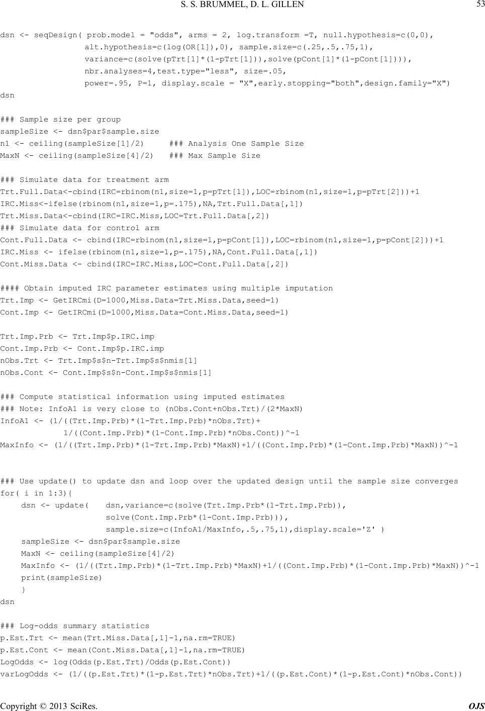

S. S. BRUMMEL, D. L. GILLEN 53
dsn <- seqDesign( prob.model = "odds", arms = 2, log.transform =T, null.hypothesis=c(0,0),
alt.hypothesis=c(log(OR[1]),0), sample.size=c(.25,.5,.75,1),
variance=c(solve(pTrt[1]*(1-pTrt[1])),solve(pCont[1]*(1-pCont[1]))),
nbr.analyses=4,test.type="less", size=.05,
power=.95, P=1, display.scale = "X",early.stopping="both",design.family="X")
dsn
### Sample size per group
sampleSize <- dsn$par$sample.size
n1 <- ceiling(sampleSize[1]/2) ### Analysis One Sample Size
MaxN <- ceiling(sampleSize[4]/2) ### Max Sample Size
### Simulate data for treatment arm
Trt.Full.Data<-cbind(IRC=rbinom(n1,size=1,p=pTrt[1]),LOC=rbinom(n1,size=1,p=pTrt[2]))+1
IRC.Miss<-ifelse(rbinom(n1,size=1,p=.175),NA,Trt.Full.Data[,1])
Trt.Miss.Data<-cbind(IRC=IRC.Miss,LOC=Trt.Full.Data[,2])
### Simulate data for control arm
Cont.Full.Data <- cbind(IRC=rbinom(n1,size=1,p=pCont[1]),LOC=rbinom(n1,size=1,p=pCont[2]))+1
IRC.Miss <- ifelse(rbinom(n1,size=1,p=.175),NA,Cont.Full.Data[,1])
Cont.Miss.Data <- cbind(IRC=IRC.Miss,LOC=Cont.Full.Data[,2])
#### Obtain imputed IRC parameter estimates using multiple imputation
Trt.Imp <- GetIRCmi(D=1000,Miss.Data=Trt.Miss.Data,seed=1)
Cont.Imp <- GetIRCmi(D=1000,Miss.Data=Cont.Miss.Data,seed=1)
Trt.Imp.Prb <- Trt.Imp$p.IRC.imp
Cont.Imp.Prb <- Cont.Imp$p.IRC.imp
nObs.Trt <- Trt.Imp$s$n-Trt.Imp$s$nmis[1]
nObs.Cont <- Cont.Imp$s$n-Cont.Imp$s$nmis[1]
### Compute statistical information using imputed estimates
### Note: InfoA1 is very close to (nObs.Cont+nObs.Trt)/(2*MaxN)
InfoA1 <- (1/((Trt.Imp.Prb)*(1-Trt.Imp.Prb)*nObs.Trt)+
1/((Cont.Imp.Prb)*(1-Cont.Imp.Prb)*nObs.Cont))^-1
MaxInfo <- (1/((Trt.Imp.Prb)*(1-Trt.Imp.Prb)*MaxN)+1/((Cont.Imp.Prb)*(1-Cont.Imp.Prb)*MaxN))^-1
### Use update() to update dsn and loop over the updated design until the sample size converges
for( i in 1:3){
dsn <- update( dsn,variance=c(solve(Trt.Imp.Prb*(1-Trt.Imp.Prb)),
solve(Cont.Imp.Prb*(1-Cont.Imp.Prb))),
sample.size=c(InfoA1/MaxInfo,.5,.75,1),display.scale='Z' )
sampleSize <- dsn$par$sample.size
MaxN <- ceiling(sampleSize[4]/2)
MaxInfo <- (1/((Trt.Imp.Prb)*(1-Trt.Imp.Prb)*MaxN)+1/((Cont.Imp.Prb)*(1-Cont.Imp.Prb)*MaxN))^-1
print(sampleSize)
}
dsn
### Log-odds summary statistics
p.Est.Trt <- mean(Trt.Miss.Data[,1]-1,na.rm=TRUE)
p.Est.Cont <- mean(Cont.Miss.Data[,1]-1,na.rm=TRUE)
LogOdds <- log(Odds(p.Est.Trt)/Odds(p.Est.Cont))
varLogOdds <- (1/((p.Est.Trt)*(1-p.Est.Trt)*nObs.Trt)+1/((p.Est.Cont)*(1-p.Est.Cont)*nObs.Cont))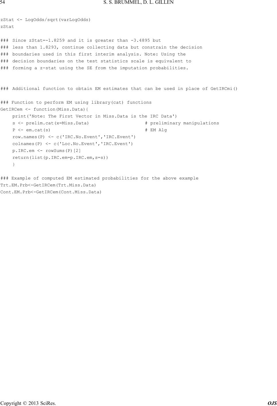

S. S. BRUMMEL, D. L. GILLEN
54
zStat <- LogOdds/sqrt(varLogOdds)
zStat
### Since zStat=-1.8259 and it is greater than -3.4895 but
### less than 1.8293, continue collecting data but constrain the decision
### boundaries used in this first interim analysis. Note: Using the
### decision boundaries on the test statistics scale is equivalent to
### forming a z-stat using the SE from the imputation probabilities.
### Additional function to obtain EM estimates that can be used in place of GetIRCmi()
### Function to perform EM using library(cat) functions
GetIRCem <- function(Miss.Data){
print('Note: The First Vector in Miss.Data is the IRC Data')
s <- prelim.cat(x=Miss.Data) # preliminary manipulations
P <- em.cat(s) # EM Alg
row.names(P) <- c('IRC.No.Event','IRC.Event')
colnames(P) <- c('Loc.No.Event','IRC.Event')
p.IRC.em <- rowSums(P)[2]
return(list(p.IRC.em=p.IRC.em,s=s))
}
### Example of computed EM estimated probabilities for the above example
Trt.EM.Prb<-GetIRCem(Trt.Miss.Data)
Cont.EM.Prb<-GetIRCem(Cont.Miss.Data)