Copy Mean: A New Method to Impute Intermittent Missing Values in Longitudinal Studies

doi:10.4236/ojs.2013.34A004

Paper Menu >>

Journal Menu >>

Open Journal of Statistics, 2013, 3, 26-40

http://dx.doi.org/10.4236/ojs.2013.34A004 Published Online August 2013 (http://www.scirp.org/journal/ojs)

Copy Mean: A New Method to Impute Intermittent

Missing Values in Longitudinal Studies

Christophe Genolini1,2*, René Écochard3,4,5, Hélène Jacqmin-Gadda6

1UMR U1027, INSERM, Université Paul Sabatier, Toulouse, France

2CeRSM (EA 2931), UFR STAPS, Université de Paris Ouest Nanterre La Défense, Nanterre, France

3Hospices Civils de Lyon, Service de Biostatistique, Lyon, France

4Université Lyon 1, Villeurbanne, France

5CNRS, UMR5558, Laboratoire de Biométrie et Biologie Evolutive, Villeurbanne, France

6Université de Bordeaux, ISPED, Centre INSERM U897-Epidemiology-Biostatistique, Bordeaux, France

Email: *christophe.genolini@u-paris10.fr

Received April 23, 2013; revised May 23, 2013; accepted May 30, 2013

cense, which permits unrestricted use, distribution, and reproduction in any medium, provided the original work is properly cited.

ABSTRACT

Longitudinal studies are those in which the same variable is repeatedly measured at different times. These studies are

more likely than others to suffer from missing values. Since the presence of missing values may have an important im-

pact on statistical analyses, it is important that they should be dealt with properly. In this paper, we present “Copy

Mean”, a new method to impute intermittent missing values. We compared its efficiency in eleven imputation methods

dedicated to the treatment of missing values in longitudinal data. All these methods were tested on three markedly dif-

ferent real datasets (stationary, increasing, and sinusoidal pattern) with complete data. For each of them, we generated

nine types of incomplete datasets that include 10%, 30%, or 50% of missing data using either a Missing Completely at

Random, a Missing at Random, or a Missing Not at Random missingness mechanism. Our results show that Copy Mean

has a great effectiveness, exceeding or equaling the performance of other methods in almost all configurations. The ef-

fectiveness of linear interpolation is highly data-dependent. The Last Occurrence Carried Forward method is strongly

discouraged.

Keywords: Imputation; Longitudinal Data; Intermittent Missing Values

1. Introduction

Longitudinal studies are those in which the same variable

is repeatedly measured at different times. They are more

likely than others to suffer from missing values [1-3].

Indeed, it is frequent that subjects miss a clinical visit or

fill out incompletely a questionnaire. The missing data

have been classified into three main categories [1]:

Missing Completely at Random (MCAR) when the mis-

singness probability is independent on the variables,

Missing at Random (MAR) when the missingness prob-

ability depends only on the observed variables, and Miss-

ing Not at Random (MNAR) when the missingness

probability may depend on unobserved variables.

When the main analysis involves statistical modeling

of the change over time of the longitudinal variable using,

for instance, mixed models, the model parameters are

generally estimated by the maximum likelihood and it is

well-known that the maximum likelihood estimation is

robust to MAR data [2,4,5]. However, selection models

and pattern-mixture models have been proposed when

the data are MNAR or when a sensitivity analysis to this

assumption is performed [2,4-7].

This paper focuses on situations where the main anal-

ysis does not involve modeling and on likelihood- based

methods such as descriptive studies, exploratory analyses,

non-parametric clustering, etc. These kinds of analyses

are very sensitive to missing data, even when the miss-

ingness mechanism is MAR; then imputation methods

are very useful.

Twisk [8] and Engels [3] compared several imputation

methods for longitudinal studies. Twisk proposed a clas-

sification of imputation methods into two categories:

“Cross-sectional” methods that impute missing values at

time t using information available at time t and “longitu-

dinal” methods that impute the missing values of an in-

dividual i using all the non-missing values of i. Engels

*Corresponding author.

C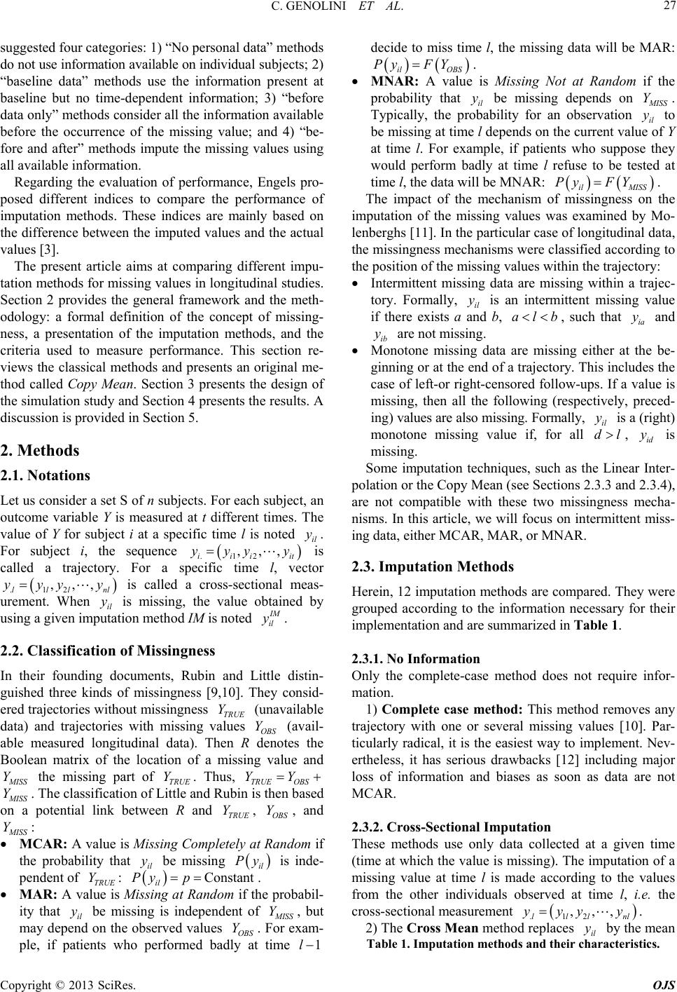. GENOLINI ET AL. 27

suggested four categories: 1) “No personal data” methods

do not use information available on individual subjects; 2)

“baseline data” methods use the information present at

baseline but no time-dependent information; 3) “before

data only” methods consider all the information available

before the occurrence of the missing value; and 4) “be-

fore and after” methods impute the missing values using

all available information.

Regarding the evaluation of performance, Engels pro-

posed different indices to compare the performance of

imputation methods. These indices are mainly based on

the difference between the imputed values and the actual

values [3].

The present article aims at comparing different impu-

tation methods for missing values in longitudinal studies.

Section 2 provides the general framework and the meth-

odology: a formal definition of the concept of missing-

ness, a presentation of the imputation methods, and the

criteria used to measure performance. This section re-

views the classical methods and presents an original me-

thod called Copy Mean. Section 3 presents the design of

the simulation study and Section 4 presents the results. A

discussion is provided in Section 5.

2. Methods

2.1. Notations

Let us consider a set S of n subjects. For each subject, an

outcome variable Y is measured at t different times. The

value of Y for subject i at a specific time l is noted il .

For subject i, the sequence



.12

,,,

iii

yy y is

called a trajectory. For a specific time l, vector



.12

,,,

llln



yy y

y is called a cross-sectional meas-

urement. When il is missing, the value obtained by

using a given imputation method IM is noted

2.2. Classification of Missingness

In their founding documents, Rubin and Little distin-

guished three kinds of missingness [9,10]. They consid-

ered trajectories without missingness TRUE (unavailable

data) and trajectories with missing values OBS

Y (avail-

able measured longitudinal data). Then R denotes the

Boolean matrix of the location of a missing value and

ISS

Y the missing part of TRUE

Y. Thus, TRUE OBS





ISS . The classification of Little and Rubin is then based

on a potential link between R and TRUE

, OB

Y, and

ISS

 MCAR: A value is Missing Comp letely at Random if

the probability that il

y be missing



Py is inde-

pendent of Y: .

TRUE il

 MAR: A value is Missing at Random if the probabil-

ity that il

y be missing is independent of



Constap ntPy

ISS

Y, but

may depend on the observed values OBS

Y. For exam-

ple, if patients who performed badly at time 1l



decide to miss time l, the missing data will be MAR:









il OBS

Py FY.

 MNAR: A value is Missing Not at Random if the

probability that il

y be missing depends on

ISS

Typically, the probability for an observation il

y to

be missing at time l depends on the current value of Y

at time l. For example, if patients who suppose they

would perform badly at time l refuse to be tested at

time l, the data will be MNAR:







il MISS

The impact of the mechanism of missingness on the

imputation of the missing values was examined by Mo-

lenberghs [11]. In the particular case of longitudinal data,

the missingness mechanisms were classified according to

the position of the missing values within the trajectory:

Py FY.

 Intermittent missing data are missing within a trajec-

tory. Formally, il

y is an intermittent missing value

if there exists a and b, alb , such that ia

y and

y are not missing.

 Monotone missing data are missing either at the be-

ginning or at the end of a trajectory. This includes the

case of left-or right-censored follow-ups. If a value is

missing, then all the following (respectively, preced-

ing) values are also missing. Formally, il

y is a (right)

monotone missing value if, for all dl, id

y is

missing.

Some imputation techniques, such as the Linear Inter-

polation or the Copy Mean (see Sections 2.3.3 and 2.3.4),

are not compatible with these two missingness mecha-

nisms. In this article, we will focus on intermittent miss-

ing data, either MCAR, MAR, or MNAR.

2.3. Imputation Methods

Herein, 12 imputation methods are compared. They were

grouped according to the information necessary for their

implementation and are summarized in Table 1.

2.3.1. No Information

Only the complete-case method does not require infor-

mation.

1) Complete case method: This method removes any

trajectory with one or several missing values [10]. Par-

ticularly radical, it is the easiest way to implement. Nev-

ertheless, it has serious drawbacks [12] including major

loss of information and biases as soon as data are not

MCAR.

2.3.2. Cross-Sectional Imputation

These methods use only data collected at a given time

(time at which the value is missing). The imputation of a

missing value at time l is made according to the values

from the other individuals observed at time l, i.e. the

cross-sectional measurement



.12

,,,

lllnl

yy y

2) The Cross Mean method replaces by the mean

Table 1. Imputation methods and their characteristics.

C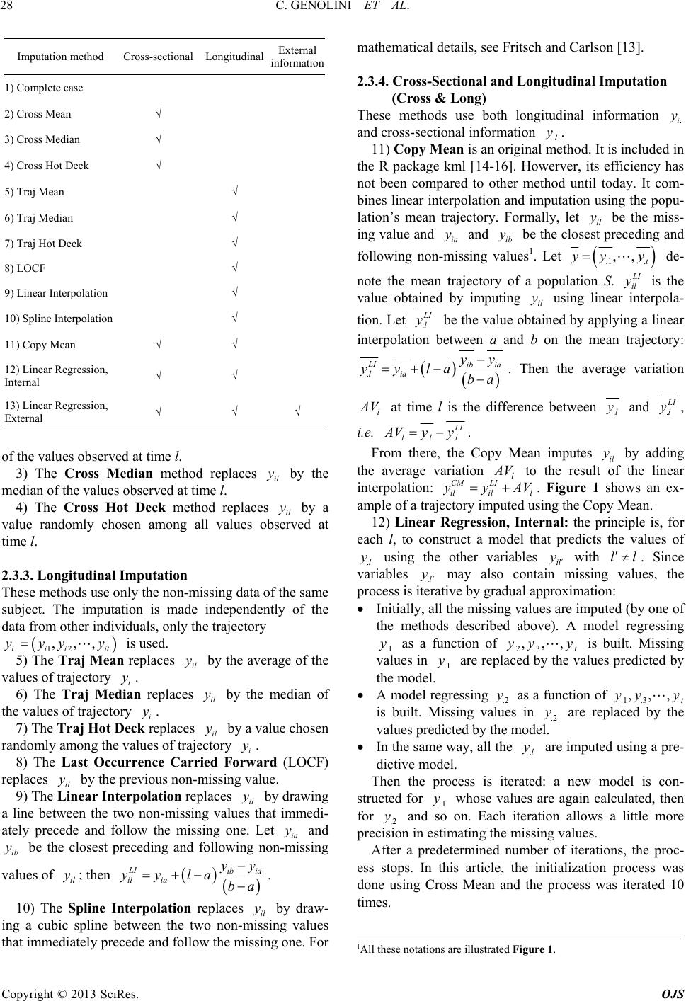. GENOLINI ET AL.

Imputation method Cross-sectional Longitudinal External

information

1) Complete case

2) Cross Mean √

3) Cross Median √

4) Cross Hot Deck √

5) Traj Mean √

6) Traj Median √

7) Traj Hot Deck √

8) LOCF √

9) Linear Interpolation √

10) Spline Interpolation √

11) Copy Mean √ √

12) Linear Regression,

Internal √ √

13) Linear Regression,

External √ √ √

of the values observed at time l.

3) The Cross Median method replaces by the

median of the values observed at time l. il

4) The Cross Hot Deck method replaces il by a

value randomly chosen among all values observed at

time l.

2.3.3. Longitudinal Imputation

These methods use only the non-missing data of the same

subject. The imputation is made independently of the

data from other individuals, only the trajectory



.12

,,,

iii it

yy y is used.

5) The Traj Mean replaces by the average of the

values of trajectory . il

6) The Traj Median replaces by the median of

the values of trajectory .

7) The Traj Hot Deck replaces il by a value chosen

randomly among the values of trajectory .

8) The Last Occurrence Carried Forward (LOCF)

replaces by the previous non-missing value.

9) The Linear Interpolation replaces il by drawing

a line between the two non-missing values that immedi-

ately precede and follow the missing one. Let ia and

be the closest preceding and following non-missing

values of ; then



LI ib ia

il iayy

yyla

 .

10) The Spline Interpolation replaces il by draw-

ing a cubic spline between the two non-missing values

that immediately precede and follow the missing one. For

mathematical details, see Fritsch and Carlson [13].

2.3.4. Cross-Sectional and Longitudinal Imputation

(Cross & Long)

These methods use both longitudinal information

and cross-sectional information . .i

11) Copy Mean is an original method. It is included in

the R package kml [14-16]. Howerver, its efficiency has

not been compared to other method until today. It com-

bines linear interpolation and imputation using the popu-

lation’s mean trajectory. Formally, let il be the miss-

ing value and and be the closest preceding and

yib

following non-missing values1. Let



.1 .

yy y de-

note the mean trajectory of a population S.

is the

value obtained by imputing using linear interpola-

tion. Let .

y be the value obtained by applying a linear

interpolation between a and b on the mean trajectory:



LI ib ia

lia

yyla



 . Then the average variation

V at time l is the difference between .l

and .

i.e. ..

lll

Vyy .

From there, the Copy Mean imputes il by adding

the average variation

LI to the result of the linear

interpolation: il il l

yAV. Figure 1 shows an ex-

ample of a trajectory imputed using the Copy Mean.

12) Linear Regression, Internal: the principle is, for

each l, to construct a model that predicts the values of

.l using the other variables il with yy l

l



. Since

variables .l



may also contain missing values, the

process is iterative by gradual approximation:

 Initially, all the missing values are imputed (by one of

the methods described above). A model regressing

y as a function of .2.3.

,,,

t is built. Missing

values in .1

y are replaced by the values predicted by

the model.

yy y

 A model regressing .2

y as a function of .1.3.

,,,

is built. Missing values in .2

y are replaced by the

values predicted by the model.

yy y

 In the same way, all the .l

y are imputed using a pre-

dictive model.

Then the process is iterated: a new model is con-

structed for .1 whose values are again calculated, then

for .2 and so on. Each iteration allows a little more

precision in estimating the missing values.

After a predetermined number of iterations, the proc-

ess stops. In this article, the initialization process was

done using Cross Mean and the process was iterated 10

times.

1All these notations are illustrated Figure 1.

C. GENOLINI ET AL.

located in Aix-en-Provence, Dijon, and Lyon (France),

Milano and Verona (Italy), DÃ1

4sseldorf (Germany),

LiÃ¨ge (Belgium) and Madrid (Spain). Urine preg-

nanediol-3a-glucuronide was measured before ovulation.

This variable is a continuous in the range [0.05; 26.6]

mg/L (Overall mean: 11.5 mg/L; overall standard devia-

tion: 18.3). The trajectories of this variable have the

characteristic of being non-stationary and increasing. Of

the 102 trajectories, two (1.96% of total) had missing

values. These trajectories were removed from the present

study. Because some imputation methods require the use

of covariates, we chose five covariates more or less cor-

related with the longitudinal variable under study: weight,

size, age at menarche, number of children, and current

age.

Figure 1. Copy Mean imputation. The individual trajectory

is in black, the mean trajectory

y is in red. The dot-

ted lines are the values imputed by linear interpolation. The

dashed lines are values imputed by Copy Mean.

2.4. Cross-Sectional and Longitudinal

Imputation using Covariables (External) Fish: The second dataset (Figure 2(b)) comes from a

study on an automatic pattern recognition system applied

to the monitoring of fish migration [18]. It included 350

individuals. The main variable is continuous in the range

[−1.83; 1.95] (overall mean: 0.16; overall standard devia-

tion: 0.89). The trajectories present some large variations

and are close to sinusoidal functions. The dataset has no

missing values but the covariates were not accessible;

thus, methods that use covariates were not tested on this

dataset.

Finally, it is possible to use all the information, including

some covariates measured at baseline:

13) Linear Regression, External: the principle is the

same as the internal linear regression (iterative process

on all cross-sectional variables) but the predictive model

for .l is a function of both other trajectories y.l



and

some covariates.

3. Simulation

Alcohol: The third dataset (Figure 2(c)) comes from

the Quebec Longitudinal Study of Child Development

led by the GRIP [19]. In this study, 1831 participants

were interviewed retrospectively; thus, the data show a

very low rate of missingness. The monthly alcohol con-

sumption was rated on a four-point scale (0 to 4, overall

mean: 1.18; overall standard deviation: 1.09). The main

feature of this study is the stability of the values over

time. Three trajectories had missing values (0.16% of

total); they were removed from the study. The covariates

selected were: sex, happiness scores, income, tobacco

consumption, and expenditure on tobacco.

3.1. Data Generation

The present simulation study was performed using three

existing datasets with complete data. Several incomplete

datasets were obtained by generating missing values ac-

cording to different schemes. To be as general as possi-

ble, we worked on three datasets with very different cha-

racteristics.

3.1.1. The Three Datasets

Pregnanediol: The first dataset (Figure 2(a)) comes

from a study on human menstrual cycles [17]. The initial

aim of the study was a search for biomarkers for accurate

prediction of ovulation. One hundred and two women

were recruited from eight natural family planning clinics

3.1.2. Generation of Missing Values

Several methods may be used to generate missing values

Figure 2. Graphical representations of the three dataset. Individual trajectories are in black. The overall mean trajectories

re in red. (a) Pregnanediol; (b) Fish; (c) Alcohol. a

C. GENOLINI ET AL.

[20]. In the present article, for each of 3 complete data-

sets, we generated 9 (3 × 3) types of incomplete datasets

that included 10%, 30%, or 50% missing data using ei-

ther a MCAR, a MAR, or a MNAR missingness mecha-

nism. This process was repeated 500 times. Thus, 13,500

datasets (3 × 9 × 500) were simulated. The incomplete

datasets on pregnanediol and alcohol were analyzed with

the 12 imputation methods. The incomplete datasets on

fish were analyzed with only the 11 methods that do not

require external data.

To generate intermittent missing values in a complete

dataset, we defined a probability function







that il be missing for l in y





2, 1t (the first and last

values were always observed ones). In the MCAR case,

this probability is independent of Y:







MCAR il

logiR b

y

t P. In the MAR case, the prob-

ability depends on il where is the last observed

value preceding il : il

y







AR il

P Ril

logitbby







.

Finally, in the MNAR case, the probability depends on

the current value :





NAR il

P Ril

bbylogit  .

3.2. Imputation Quality Comparison Criteria

To assess the quality of the different imputation methods,

we considered the deviation which is the difference be-

tween the true and the imputed value [3] The deviation

then leads to three criteria: 1) the Bias is the mean of the

deviation; 2) the Mean Absolute Deviation (MAD) is

the average of the absolute deviations; and, 3) the Root

Mean Square Deviation (RMSD) is the square root of

the mean of the square of the deviation. When il is the

real value that method IM imputed as

, the Bias is

il il



, the MAD is

il il



 and the RMSD



il il



, m being the total number of miss-

ing values.

3.3. Methods and Softwares

All the analyses were performed with R software [21].

Classical and new imputation methods have been pro-

grammed and published in package Longitudinal Data on

CRAN [22]. The spline imputation method was pro-

grammed using stats package [13,23]. Imputations need-

ing linear regression used function mice (mice package)

with method “predictive mean matching” [24].

4. Results

During data construction, three mechanisms of missing-

ness (MCAR, MAR, and MNAR), three percentages of

missing data (10%, 30%, and 50%) and three types of

data (Pregnanediol, Fish, and Alcohol) were considered.

The analysis of the results showed that the missingness

mechanism and the type of dataset had impacts on the

performance of the methods but not the percentage of

missing data. Thus, for brevity, only the tables relative to

30% missing data will be presented in the main text. The

full results are given in the Appendix.

4.1. Mean Absolute Deviation Results

The Mean Absolute Deviation (MAD) is the average of

the absolute deviations between the real values and the

imputed values. Table 2 presents the mean result for

each method according to the missingness mechanism

and the type of dataset. For better readability, the results

were standardized: in each case (each column) the per-

formance of the best method (the lowest MAD) was set

to 1 so that all other results are multiples of this reference

value. In Table 2, the performances of the “good meth-

ods” are highlighted in bold. The “good methods” are

those whose values are between 1 and 1.2. The threshold

of 1.2 was chosen arbitrarily.

With Pregnanediol data, Copy Mean, Linear Interpola-

tion, LOCF, Traj Median and Traj Mean, were the best.

With Fish data, the most effective methods were Copy

Mean, Linear Regression Internal, Cross Median, and

Cross Mean. All methods that use only longitudinal in-

formation performed poorly with this data set character-

ized by a strong non-linear trend with low inter-subject

variability (see Figure 2(b)). With Alcohol data, Linear

Interpolation and Copy Mean gave the best results.

There were no marked differences between MCAR,

MAR, and MNAR. Only the Spline Interpolation method

performed poorly with MAR on Alcohol dataset. This

was probably due to the fact that, with MAR, long series

of contiguous missing values are more likely; in such a

case, the Spline Interpolation method imputes by poly-

nomials with values far from the original curve.

4.2. Root Mean Square Deviation Results

Table 3 presents the root mean square deviation results.

Here too, the results were standardized. The performance

of the best method (the lowests RMSD) was set to 1 so

that all other results are multiples of this reference value.

In Table 3, the hight performance values (1.4 or lower)

are highlighted in bold. The threshold of 1.4 was chosen

arbitrarily. The results with the Root Mean Square De-

viation were close to those obtained with the MAD crite-

rion. They are detailed in the Appendix.

4.3. Bias Results

Table 4 presents the results for bias. The “good methods”

(between −0.03 and 0.03) are highlighted in bold. The

hresholds of −0.03 and +0.03 were arbitrarily chosen. t

C. GENOLINI ET AL. 31

Table 2. MAD (Mean Absolute Deviations) according to the imputation method in each dataset.

Pregnanediol Fish Alcohol

Imputation method

MCAR MAR MNAR MCAR MAR MNAR MCAR MAR MNAR

1) Cross Mean 1.38 1.31 1.46 1.26 1.19 1.17 6.30 5.05 4.63

2) Cross Median 1.28 1.21 1.47 1.25 1.17 1.15 5.95 5.17 4.82

3) Cross Hot Deck 1.84 1.74 1.88 1.79 1.69 1.65 8.06 6.51 5.94

4) Traj Mean 1.31 1.16 1.25 4.94 5.09 5.33 4.39 3.74 3.55

5) Traj Median 1.26 1.15 1.35 5.09 5.19 5.52 3.81 3.67 3.57

6) Traj Hot Deck 1.73 1.51 1.64 6.58 6.51 6.59 4.83 4.05 3.77

7) LOCF 1.11 1.12 1.20 3.97 4.03 3.71 1.07 1.33 1.31

8) Linear Interpolation 1 1.01 1 1.66 1.83 2.03 1 1 1

9) Spline Interpolation 1.59 1.74 1.43 1.54 1.80 1.78 1.59 6.40 1.87

10) Copy Mean 1 1 1.06 1 1 1 1.11 1.12 1.10

11) Linear Regression, Internal 1.39 1.31 1.46 1.26 1.19 1.18 6.28 5.06 4.64

12) Linear Regression, External 1.48 1.43 1.50 NA NA NA 1.59 1.61 1.51

Table 3. RMSD (Root Mean Scare Deviations) according to the imputation method in each dataset.

Pregnanediol Fish Alcohol

Imputation method

MCAR MAR MNAR MCAR MAR MNAR MCAR MAR MNAR

1) Cross Mean 1.51 1.38 1.81 1.55 1.32 1.31 7.34 5.75 5.09

2) Cross Median 1.68 1.54 2.18 1.58 1.33 1.31 8.69 7.5 6.74

3) Cross Hot Deck 2.96 2.75 3.08 3.1 2.64 2.6 14.6 10.8 9.33

4) Traj Mean 1.38 1.17 1.41 17.9 17.4 19.52 4.67 4.05 3.83

5) Traj Median 1.6 1.4 1.85 18.9 18.2 20.84 6.51 6.03 5.56

6) Traj Hot Deck 2.85 2.3 2.57 34.4 32.1 33.76 9.16 7.03 6.19

7) LOCF 1.36 1.33 1.52 12.3 13.5 11.09 1.83 2.14 1.99

8) Linear Interpolation 1 1.04 1 2.78 3.36 3.95 1 1 1

9) Spline Interpolation 3.19 4.03 2.44 2.53 4.34 4.26 1.81 185.5 8.92

10) Copy Mean 1 1 1.08 1 1 1 1 1.03 1

11) Linear Regression, Internal 1.55 1.37 1.79 1.55 1.33 1.33 7.31 5.75 5.1

12) Linear Regression, External 1.94 1.88 2 NA NA NA 2.01 1.94 1.77

Most methods had little or no bias: 60.2% had a bias

ranging between −0.03 and +0.03 and 69.9% a bias be-

tween −0.05 and +0.05. There were important differences

in bias between MCAR, MAR, and MNAR mechanisms.

The bias was slightly larger with the MAR than with the

MCAR and even larger with MNAR (see Table 4). This

is due to the fact that in MAR and in MNAR mechanisms,

the low values are those that are the most likely missing.

4.4. Summary

Table 5 summarizes the results obtained with all the

methods and criteria. Each column shows how many

times a method has been particularly performant accord-

ing to the above-defined criteria (Tables 2-4).

5. Discussion

In this article, we compare different methods for imput-

ing trajectories. Missing data were generated according

three different mechanisms (MCAR, MAR, and MNAR)

in three dataset exhibiting strong structural differences.

Eleven conventional methods and one original technique

were compared according to three performance criteria:

the Mean Absolute Deviation, the Root Square Mean

Deviation, and Bias.

C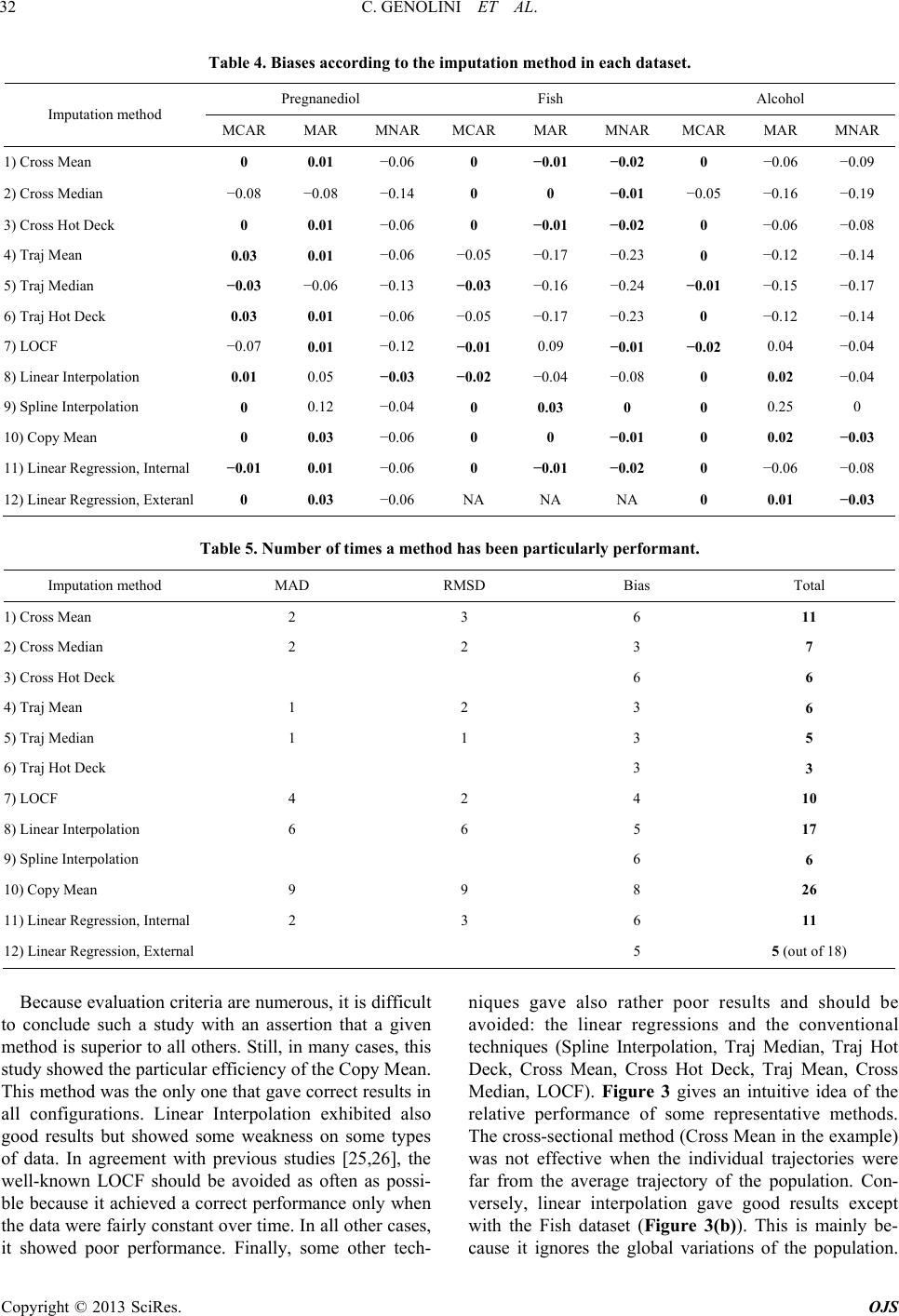. GENOLINI ET AL.

Table 4. Biases according to the imputation method in each dataset.

Pregnanediol Fish Alcohol

Imputation method

MCAR MAR MNAR MCAR MAR MNAR MCAR MAR MNAR

1) Cross Mean 0 0.01 −0.06 0 −0.01 −0.02 0 −0.06 −0.09

2) Cross Median −0.08 −0.08 −0.14 0 0 −0.01 −0.05 −0.16 −0.19

3) Cross Hot Deck 0 0.01 −0.06 0 −0.01 −0.02 0 −0.06 −0.08

4) Traj Mean 0.03 0.01 −0.06 −0.05 −0.17 −0.23 0 −0.12 −0.14

5) Traj Median −0.03 −0.06 −0.13 −0.03 −0.16 −0.24 −0.01 −0.15 −0.17

6) Traj Hot Deck 0.03 0.01 −0.06 −0.05 −0.17 −0.23 0 −0.12 −0.14

7) LOCF −0.07 0.01 −0.12 −0.01 0.09 −0.01 −0.02 0.04 −0.04

8) Linear Interpolation 0.01 0.05 −0.03 −0.02 −0.04 −0.08 0 0.02 −0.04

9) Spline Interpolation 0 0.12 −0.04 0 0.03 0 0 0.25 0

10) Copy Mean 0 0.03 −0.06 0 0 −0.01 0 0.02 −0.03

11) Linear Regression, Internal −0.01 0.01 −0.06 0 −0.01 −0.02 0 −0.06 −0.08

12) Linear Regression, Exteranl 0 0.03 −0.06 NA NA NA 0 0.01 −0.03

Table 5. Number of times a method has been particularly performant.

Imputation method MAD RMSD Bias Total

1) Cross Mean 2 3 6 11

2) Cross Median 2 2 3 7

3) Cross Hot Deck 6 6

4) Traj Mean 1 2 3 6

5) Traj Median 1 1 3 5

6) Traj Hot Deck 3 3

7) LOCF 4 2 4

8) Linear Interpolation 6 6 5 17

9) Spline Interpolation 6 6

10) Copy Mean 9 9 8 26

11) Linear Regression, Internal 2 3 6 11

12) Linear Regression, External 5 5 (out of 18)

Because evaluation criteria are numerous, it is difficult

to conclude such a study with an assertion that a given

method is superior to all others. Still, in many cases, this

study showed the particular efficiency of the Copy Mean.

This method was the only one that gave correct results in

all configurations. Linear Interpolation exhibited also

good results but showed some weakness on some types

of data. In agreement with previous studies [25,26], the

well-known LOCF should be avoided as often as possi-

ble because it achieved a correct performance only when

the data were fairly constant over time. In all other cases,

it showed poor performance. Finally, some other tech-

niques gave also rather poor results and should be

avoided: the linear regressions and the conventional

techniques (Spline Interpolation, Traj Median, Traj Hot

Deck, Cross Mean, Cross Hot Deck, Traj Mean, Cross

Median, LOCF). Figure 3 gives an intuitive idea of the

relative performance of some representative methods.

The cross-sectional method (Cross Mean in the example)

was not effective when the individual trajectories were

far from the average trajectory of the population. Con-

versely, linear interpolation gave good results except

with the Fish dataset (Figure 3(b)). This is mainly be-

cause it ignores the global variations of the population.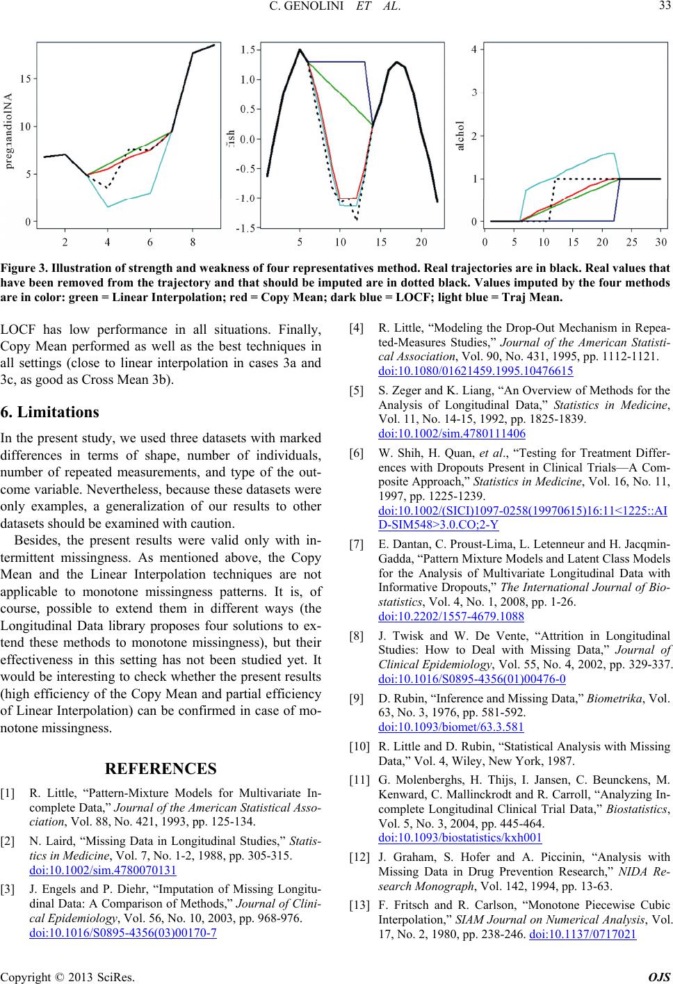

C. GENOLINI ET AL. 33

Figure 3. Illustration of strength and weakness of four representatives method. Real trajectories are in black. Real values that

have been removed from the trajectory and that should be imputed are in dotted black. Values imputed by the four methods

are in color: green = Linear Interpolation; red = Copy Mean; dark blue = LOCF; light blue = Traj Mean.

LOCF has low performance in all situations. Finally,

Copy Mean performed as well as the best techniques in

all settings (close to linear interpolation in cases 3a and

3c, as good as Cross Mean 3b).

6. Limitations

In the present study, we used three datasets with marked

differences in terms of shape, number of individuals,

number of repeated measurements, and type of the out-

come variable. Nevertheless, because these datasets were

only examples, a generalization of our results to other

datasets should be examined with caution.

Besides, the present results were valid only with in-

termittent missingness. As mentioned above, the Copy

Mean and the Linear Interpolation techniques are not

applicable to monotone missingness patterns. It is, of

course, possible to extend them in different ways (the

Longitudinal Data library proposes four solutions to ex-

tend these methods to monotone missingness), but their

effectiveness in this setting has not been studied yet. It

would be interesting to check whether the present results

(high efficiency of the Copy Mean and partial efficiency

of Linear Interpolation) can be confirmed in case of mo-

notone missingness.

REFERENCES

[1] R. Little, “Pattern-Mixture Models for Multivariate In-

complete Data,” Journal of the American Statistical Asso-

ciation, Vol. 88, No. 421, 1993, pp. 125-134.

[2] N. Laird, “Missing Data in Longitudinal Studies,” Statis-

tics in Medicine, Vol. 7, No. 1-2, 1988, pp. 305-315.

doi:10.1002/sim.4780070131

[3] J. Engels and P. Diehr, “Imputation of Missing Longitu-

dinal Data: A Comparison of Methods,” Journal of Clini-

cal Epidemiology, Vol. 56, No. 10, 2003, pp. 968-976.

doi:10.1016/S0895-4356(03)00170-7

[4] R. Little, “Modeling the Drop-Out Mechanism in Repea-

ted-Measures Studies,” Journal of the American Statisti-

cal Association, Vol. 90, No. 431, 1995, pp. 1112-1121.

doi:10.1080/01621459.1995.10476615

[5] S. Zeger and K. Liang, “An Overview of Methods for the

Analysis of Longitudinal Data,” Statistics in Medicine,

Vol. 11, No. 14-15, 1992, pp. 1825-1839.

doi:10.1002/sim.4780111406

[6] W. Shih, H. Quan, et al., “Testing for Treatment Differ-

ences with Dropouts Present in Clinical Trials—A Com-

posite Approach,” Statistics in Medicine, Vol. 16, No. 11,

1997, pp. 1225-1239.

doi:10.1002/(SICI)1097-0258(19970615)16:11<1225::AI

D-SIM548>3.0.CO;2-Y

[7] E. Dantan, C. Proust-Lima, L. Letenneur and H. Jacqmin-

Gadda, “Pattern Mixture Models and Latent Class Models

for the Analysis of Multivariate Longitudinal Data with

Informative Dropouts,” The International Journal of Bio-

statistics, Vol. 4, No. 1, 2008, pp. 1-26.

doi:10.2202/1557-4679.1088

[8] J. Twisk and W. De Vente, “Attrition in Longitudinal

Studies: How to Deal with Missing Data,” Journal of

Clinical Epidemiology, Vol. 55, No. 4, 2002, pp. 329-337.

doi:10.1016/S0895-4356(01)00476-0

[9] D. Rubin, “Inference and Missing Data,” Biometrika, Vol.

63, No. 3, 1976, pp. 581-592.

doi:10.1093/biomet/63.3.581

[10] R. Little and D. Rubin, “Statistical Analysis with Missing

Data,” Vol. 4, Wiley, New York, 1987.

[11] G. Molenberghs, H. Thijs, I. Jansen, C. Beunckens, M.

Kenward, C. Mallinckrodt and R. Carroll, “Analyzing In-

complete Longitudinal Clinical Trial Data,” Biostatistics,

Vol. 5, No. 3, 2004, pp. 445-464.

doi:10.1093/biostatistics/kxh001

[12] J. Graham, S. Hofer and A. Piccinin, “Analysis with

Missing Data in Drug Prevention Research,” NIDA Re-

search Monograph, Vol. 142, 1994, pp. 13-63.

[13] F. Fritsch and R. Carlson, “Monotone Piecewise Cubic

Interpolation,” SIAM Journal on Numerical Analysis, Vol.

17, No. 2, 1980, pp. 238-246. doi:10.1137/0717021

C. GENOLINI ET AL.

[14] C. Genolini and B. Falissard, “Kml: k-Means for Longitu-

dinal Data,” Computational Statistics, Vol. 25, No. 2,

2010, pp. 317-328. doi:10.1007/s00180-009-0178-4

[15] C. Genolini and B. Falissard, “Kml: A Package to Cluster

Longitudinal Data,” Computer Methods and Programs in

Biomedicine, Vol. 104, No. 3, 2011, pp. e112-e121.

doi:10.1016/j.cmpb.2011.05.008

[16] C. Genolini, J. Pingault, T. Driss, S. Côté, R. Tremblay, F.

Vitaro, C. Arnaud and B. Falissard, “KmL3D: A Non-Pa-

rametric Algorithm for Clustering Joint Trajectories,”

Computer Methods and Programs in Biomedicine, Vol.

109, No. 1, 2012, pp. 104-111.

[17] R. Ecochard, H. Boehringer, M. Rabilloud and H. Marret,

“Chronological Aspects of Ultrasonic, Hormonal, and

Other Indirect Indices of Ovulation,” BJOG: An Interna-

tional Journal of Obstetrics & Gynaecology, Vol. 108,

No. 8, 2001, pp. 822-829.

doi:10.1111/j.1471-0528.2001.00194.x

[18] D. Lee, J. Archibald, R. Schoenberger, A. Dennis and D.

Shiozawa, “Contour Matching for Fish Species Recogni-

tion and Migration Monitoring,” Applications of Compu-

tational Intelligence in Biology, Vol. 122, 2008, pp. 183-

207.

[19] R. Tremblay, R. Pihl, F. Vitaro, and P. Dobkin, “Predict-

ing Early Onset of Male Antisocial Behavior from Pre-

school Behavior,” Archives of General Psychiatry, Vol.

51, No. 9, 1994, p. 732.

doi:10.1001/archpsyc.1994.03950090064009

[20] O. François and P. Leray, “Generation of Incompliete

Test-Data Usinng Bayesinan Networks,” International

Joint Conference on Neural Networks, Orlando, 12-17

August 2007, pp. 2391-2396.

[21] R Development Core Team, “A Language and Environ-

ment for Statistical Computing,” R Foundation for Statis-

tical Computing, Vienna, 2012.

[22] C. Genolini, “Longitudinal Data,” R Package Version 2.3.,

2012.

[23] G. Forsythe, M. Malcolm and C. Moler, “Computer Me-

thods for Mathematical Computations,” Prentice Hall

Professional Technical Reference, 1977.

[24] S. Buuren and K. Groothuis-Oudshoorn, “Mice: Multi-

variate Imputation by Chained Equations in r,” Journal of

Statistical Software, Vol. 45, No. 3, 2011.

[25] G. Gadbury, C. Coffey and D. Allison, “Modern Statis-

tical Methods for Handling Missing Repeated Measure-

ments in Obesity Trial Data: Beyond LOCF,” Obesity

Reviews, Vol. 4, No. 3, 2003, pp. 175-184.

doi:10.1046/j.1467-789X.2003.00109.x

[26] S. Fielding, G. Maclennan, J. Cook and C. Ramsay, “A

Review of RCTS in Four Medical Journals to Assess the

Use of Imputation to Overcome Missing Data in Quality

of Life Outcomes,” Trials, Vol. 9, No. 1, 2008, p. 51.

doi:10.1186/1745-6215-9-51

C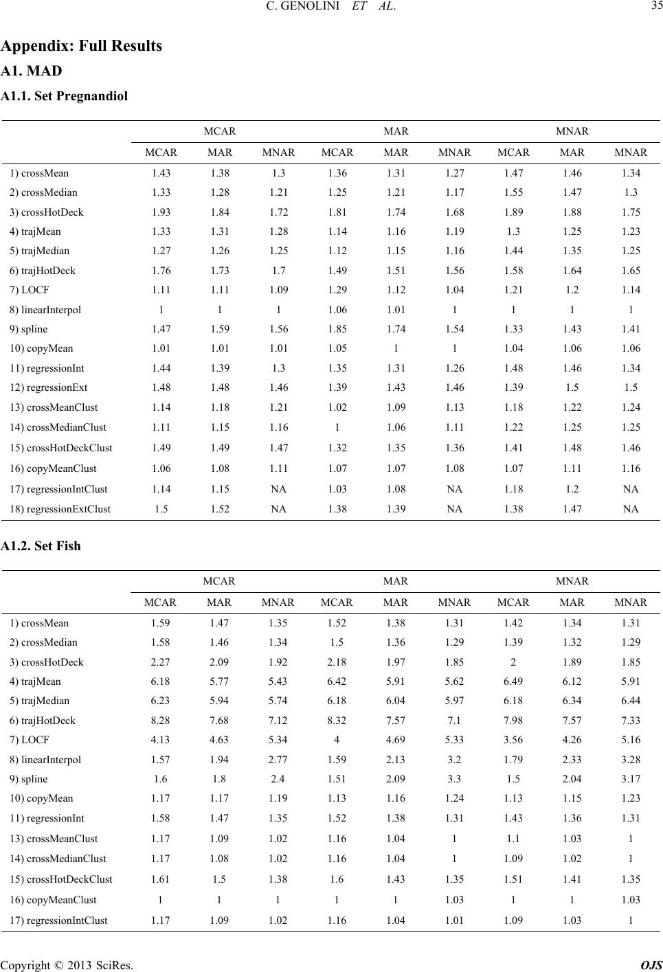. GENOLINI ET AL. 35

Appendix: Full Results

A1. MAD

A1.1. Set Pregnandiol

MCAR MAR MNAR

MCAR MAR MNAR MCAR MAR MNAR MCAR MAR MNAR

1) crossMean 1.43 1.38 1.3 1.36 1.31 1.27 1.47 1.46 1.34

2) crossMedian 1.33 1.28 1.21 1.25 1.21 1.17 1.55 1.47 1.3

3) crossHotDeck 1.93 1.84 1.72 1.81 1.74 1.68 1.89 1.88 1.75

4) trajMean 1.33 1.31 1.28 1.14 1.16 1.19 1.3 1.25 1.23

5) trajMedian 1.27 1.26 1.25 1.12 1.15 1.16 1.44 1.35 1.25

6) trajHotDeck 1.76 1.73 1.7 1.49 1.51 1.56 1.58 1.64 1.65

7) LOCF 1.11 1.11 1.09 1.29 1.12 1.04 1.21 1.2 1.14

8) linearInterpol 1 1 1 1.06 1.01 1 1 1 1

9) spline 1.47 1.59 1.56 1.85 1.74 1.54 1.33 1.43 1.41

10) copyMean 1.01 1.01 1.01 1.05 1 1 1.04 1.06 1.06

11) regressionInt 1.44 1.39 1.3 1.35 1.31 1.26 1.48 1.46 1.34

12) regressionExt 1.48 1.48 1.46 1.39 1.43 1.46 1.39 1.5 1.5

13) crossMeanClust 1.14 1.18 1.21 1.02 1.09 1.13 1.18 1.22 1.24

14) crossMedianClust 1.11 1.15 1.16 1 1.06 1.11 1.22 1.25 1.25

15) crossHotDeckClust 1.49 1.49 1.47 1.32 1.35 1.36 1.41 1.48 1.46

16) copyMeanClust 1.06 1.08 1.11 1.07 1.07 1.08 1.07 1.11 1.16

17) regressionIntClust 1.14 1.15 NA 1.03 1.08 NA 1.18 1.2 NA

18) regressionExtClust 1.5 1.52 NA 1.38 1.39 NA 1.38 1.47 NA

A1.2. Set Fish

MCAR MAR MNAR

MCAR MAR MNAR MCAR MAR MNAR MCAR MAR MNAR

1) crossMean 1.59 1.47 1.35 1.52 1.38 1.31 1.42 1.34 1.31

2) crossMedian 1.58 1.46 1.34 1.5 1.36 1.29 1.39 1.32 1.29

3) crossHotDeck 2.27 2.09 1.92 2.18 1.97 1.85 2 1.89 1.85

4) trajMean 6.18 5.77 5.43 6.42 5.91 5.62 6.49 6.12 5.91

5) trajMedian 6.23 5.94 5.74 6.18 6.04 5.97 6.18 6.34 6.44

6) trajHotDeck 8.28 7.68 7.12 8.32 7.57 7.1 7.98 7.57 7.33

7) LOCF 4.13 4.63 5.34 4 4.69 5.33 3.56 4.26 5.16

8) linearInterpol 1.57 1.94 2.77 1.59 2.13 3.2 1.79 2.33 3.28

9) spline 1.6 1.8 2.4 1.51 2.09 3.3 1.5 2.04 3.17

10) copyMean 1.17 1.17 1.19 1.13 1.16 1.24 1.13 1.15 1.23

11) regressionInt 1.58 1.47 1.35 1.52 1.38 1.31 1.43 1.36 1.31

13) crossMeanClust 1.17 1.09 1.02 1.16 1.04 1 1.1 1.03 1

14) crossMedianClust 1.17 1.08 1.02 1.16 1.04 1 1.09 1.02 1

15) crossHotDeckClust 1.61 1.5 1.38 1.6 1.43 1.35 1.51 1.41 1.35

16) copyMeanClust 1 1 1 1 1 1.03 1 1 1.03

17) regressionIntClust 1.17 1.09 1.02 1.16 1.04 1.01 1.09 1.03 1

C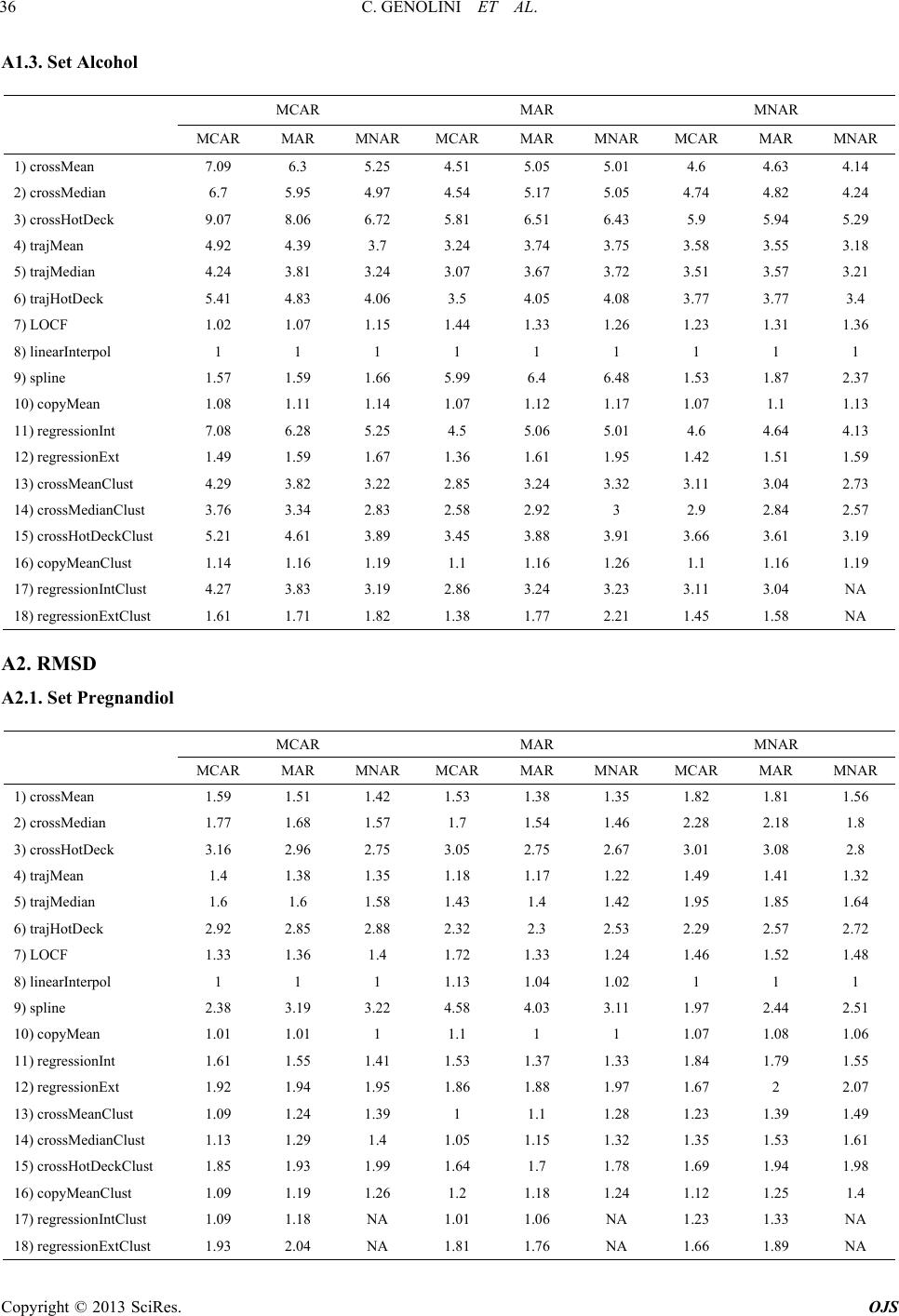. GENOLINI ET AL.

A1.3. Set Alcohol

MCAR MAR MNAR

MCAR MAR MNAR MCAR MAR MNAR MCAR MAR MNAR

1) crossMean 7.09 6.3 5.25 4.51 5.05 5.01 4.6 4.63 4.14

2) crossMedian 6.7 5.95 4.97 4.54 5.17 5.05 4.74 4.82 4.24

3) crossHotDeck 9.07 8.06 6.72 5.81 6.51 6.43 5.9 5.94 5.29

4) trajMean 4.92 4.39 3.7 3.24 3.74 3.75 3.58 3.55 3.18

5) trajMedian 4.24 3.81 3.24 3.07 3.67 3.72 3.51 3.57 3.21

6) trajHotDeck 5.41 4.83 4.06 3.5 4.05 4.08 3.77 3.77 3.4

7) LOCF 1.02 1.07 1.15 1.44 1.33 1.26 1.23 1.31 1.36

8) linearInterpol 1 1 1 1 1 1 1 1 1

9) spline 1.57 1.59 1.66 5.99 6.4 6.48 1.53 1.87 2.37

10) copyMean 1.08 1.11 1.14 1.07 1.12 1.17 1.07 1.1 1.13

11) regressionInt 7.08 6.28 5.25 4.5 5.06 5.01 4.6 4.64 4.13

12) regressionExt 1.49 1.59 1.67 1.36 1.61 1.95 1.42 1.51 1.59

13) crossMeanClust 4.29 3.82 3.22 2.85 3.24 3.32 3.11 3.04 2.73

14) crossMedianClust 3.76 3.34 2.83 2.58 2.92 3 2.9 2.84 2.57

15) crossHotDeckClust 5.21 4.61 3.89 3.45 3.88 3.91 3.66 3.61 3.19

16) copyMeanClust 1.14 1.16 1.19 1.1 1.16 1.26 1.1 1.16 1.19

17) regressionIntClust 4.27 3.83 3.19 2.86 3.24 3.23 3.11 3.04 NA

18) regressionExtClust 1.61 1.71 1.82 1.38 1.77 2.21 1.45 1.58 NA

A2. RMSD

A2.1. Set Pregnandiol

MCAR MAR MNAR

MCAR MAR MNAR MCAR MAR MNAR MCAR MAR MNAR

1) crossMean 1.59 1.51 1.42 1.53 1.38 1.35 1.82 1.81 1.56

2) crossMedian 1.77 1.68 1.57 1.7 1.54 1.46 2.28 2.18 1.8

3) crossHotDeck 3.16 2.96 2.75 3.05 2.75 2.67 3.01 3.08 2.8

4) trajMean 1.4 1.38 1.35 1.18 1.17 1.22 1.49 1.41 1.32

5) trajMedian 1.6 1.6 1.58 1.43 1.4 1.42 1.95 1.85 1.64

6) trajHotDeck 2.92 2.85 2.88 2.32 2.3 2.53 2.29 2.57 2.72

7) LOCF 1.33 1.36 1.4 1.72 1.33 1.24 1.46 1.52 1.48

8) linearInterpol 1 1 1 1.13 1.04 1.02 1 1 1

9) spline 2.38 3.19 3.22 4.58 4.03 3.11 1.97 2.44 2.51

10) copyMean 1.01 1.01 1 1.1 1 1 1.07 1.08 1.06

11) regressionInt 1.61 1.55 1.41 1.53 1.37 1.33 1.84 1.79 1.55

12) regressionExt 1.92 1.94 1.95 1.86 1.88 1.97 1.67 2 2.07

13) crossMeanClust 1.09 1.24 1.39 1 1.1 1.28 1.23 1.39 1.49

14) crossMedianClust 1.13 1.29 1.4 1.05 1.15 1.32 1.35 1.53 1.61

15) crossHotDeckClust 1.85 1.93 1.99 1.64 1.7 1.78 1.69 1.94 1.98

16) copyMeanClust 1.09 1.19 1.26 1.2 1.18 1.24 1.12 1.25 1.4

17) regressionIntClust 1.09 1.18 NA 1.01 1.06 NA 1.23 1.33 NA

18) regressionExtClust 1.93 2.04 NA 1.81 1.76 NA 1.66 1.89 NA

C. GENOLINI ET AL. 37

A2.2. Set Fish

MCAR MAR MNAR

MCAR MAR MNAR MCAR MAR MNAR MCAR MAR MNAR

1) crossMean 2.43 2.07 1.89 2.16 1.89 1.81 1.96 1.85 1.82

2) crossMedian 2.47 2.1 1.92 2.17 1.9 1.83 1.96 1.85 1.82

3) crossHotDeck 4.83 4.12 3.74 4.34 3.77 3.58 3.83 3.66 3.6

4) trajMean 27.33 23.79 22.68 27.33 24.94 24.26 28.47 27.47 26.89

5) trajMedian 27.88 25.25 25.44 25.31 25.97 27.46 25.88 29.34 31.78

6) trajHotDeck 53.2 45.78 42.33 52.83 45.82 42.73 51.07 47.52 45.27

7) LOCF 12 16.46 24.22 11.88 19.28 26.09 9.36 15.61 23.6

8) linearInterpol 2.28 3.69 8.52 2.23 4.79 11.55 2.81 5.56 11.57

9) spline 2.36 3.37 9.55 2.25 6.19 22.35 2.29 6 20.04

10) copyMean 1.33 1.33 1.54 1.25 1.43 1.75 1.24 1.41 1.71

11) regressionInt 2.38 2.06 1.89 2.17 1.89 1.81 1.96 1.87 1.83

13) crossMeanClust 1.2 1.05 1 1.16 1 1 1.07 1 1.01

14) crossMedianClust 1.22 1.06 1.01 1.18 1.02 1.01 1.08 1.01 1.02

15) crossHotDeckClust 2.28 1.99 1.84 2.21 1.88 1.81 2.06 1.9 1.83

16) copyMeanClust 1 1 1.08 1 1.06 1.18 1 1.06 1.18

17) regressionIntClust 1.2 1.05 1 1.16 1 1.01 1.07 1 1

A2.3. Set Alcohol

MCAR MAR MNAR

MCAR MAR MNAR MCAR MAR MNAR MCAR MAR MNAR

1) crossMean 8.38 7.39 6.03 5.13 5.75 5.73 4.86 5.09 4.49

2) crossMedian 9.92 8.75 7.16 6.35 7.5 7.41 6.2 6.74 5.87

3) crossHotDeck 16.75 14.77 12.04 9.69 10.84 10.8 8.88 9.33 8.22

4) trajMean 5.28 4.7 3.91 3.43 4.05 4.17 3.73 3.83 3.44

5) trajMedian 7.35 6.55 5.41 4.98 6.03 6.19 5.2 5.56 5

6) trajHotDeck 10.39 9.22 7.59 6.09 7.03 7.16 5.94 6.19 5.53

7) LOCF 1.75 1.84 1.96 2.38 2.14 2.02 1.78 1.99 2.06

8) linearInterpol 1 1.01 1 1 1 1 1 1 1

9) spline 1.54 1.82 2.67 179.22 185.59 174.71 4.26 8.92 15.19

10) copyMean 1 1.01 1 1.03 1.03 1.04 1 1 1.01

11) regressionInt 8.37 7.36 6.02 5.12 5.75 5.73 4.86 5.1 4.48

12) regressionExt 1.95 2.03 2.08 1.73 1.94 2.28 1.63 1.77 1.84

13) crossMeanClust 3.85 3.41 2.86 2.52 2.86 2.89 2.75 2.73 2.4

14) crossMedianClust 4.59 4.07 3.39 2.96 3.37 3.49 3.2 3.24 2.94

15) crossHotDeckClust 7.43 6.53 5.38 4.46 5.03 5.07 4.39 4.48 3.93

16) copyMeanClust 1.01 1 1.01 1.04 1.04 1.08 1.01 1.02 1.04

17) regressionIntClust 3.84 3.41 2.85 2.52 2.87 2.88 2.74 2.74 NA

18) regressionExtClust 2.03 2.13 2.32 1.65 2.09 2.65 1.61 1.83 NA

C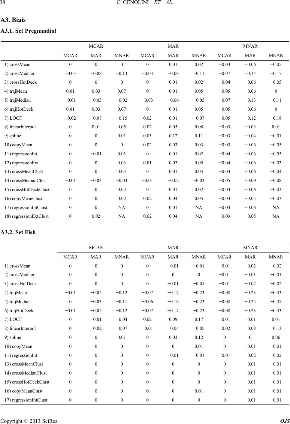. GENOLINI ET AL.

A3. Biais

A3.1. Set Pregnandiol

MCAR MAR MNAR

MCAR MAR MNAR MCAR MAR MNAR MCAR MAR MNAR

1) crossMean 0 0 0 0 0.01 0.02 −0.03 −0.06 −0.05

2) crossMedian −0.03 −0.08 −0.13 −0.03 −0.08 −0.11 −0.07 −0.14 −0.17

3) crossHotDeck 0 0 0 0 0.01 0.02 −0.04 −0.06 −0.05

4) trajMean 0.01 0.03 0.07 0 0.01 0.05 −0.05 −0.06 0

5) trajMedian −0.01 −0.03 −0.02 −0.03 −0.06 −0.05 −0.07 −0.13 −0.11

6) trajHotDeck 0.01 0.03 0.07 0 0.01 0.05 −0.05 −0.06 0

7) LOCF −0.02 −0.07 −0.15 0.02 0.01 −0.07 −0.05 −0.12 −0.18

8) linearInterpol 0 0.01 0.05 0.02 0.05 0.08 −0.03 −0.03 0.01

9) spline 0 0 0.01 0.05 0.12 0.11 −0.03 −0.04 −0.01

10) copyMean 0 0 0 0.02 0.03 0.03 −0.03 −0.06 −0.05

11) regressionInt 0 −0.01 0.01 0 0.01 0.02 −0.04 −0.06 −0.05

12) regressionExt 0 0 0.03 0.01 0.03 0.05 −0.04 −0.06 −0.03

13) crossMeanClust 0 0 0.03 0 0.01 0.03 −0.04 −0.06 −0.04

14) crossMedianClust −0.01 −0.03 −0.03 −0.01 −0.02 −0.03 −0.05 −0.09 −0.08

15) crossHotDeckClust 0 0 0.02 0 0.01 0.02 −0.04 −0.06 −0.03

16) copyMeanClust 0 0 0.02 0.02 0.04 0.05 −0.03 −0.05 −0.03

17) regressionIntClust 0 0 NA 0 0.01 NA −0.04 −0.06 NA

18) regressionExtClust 0 0.02 NA 0.02 0.04 NA −0.03 −0.05 NA

A3.2. Set Fish

MCAR MAR MNAR

MCAR MAR MNAR MCAR MAR MNAR MCAR MAR MNAR

1) crossMean 0 0 0 0 −0.01 −0.01 −0.01 −0.02 −0.02

2) crossMedian 0 0 0 0 0 0 −0.01 −0.01 −0.01

3) crossHotDeck 0 0 0 0 −0.01 −0.01 −0.01 −0.02 −0.02

4) trajMean −0.01 −0.05 −0.12 −0.07 −0.17 −0.23 −0.08 −0.23 −0.33

5) trajMedian 0 −0.03 −0.11 −0.06 −0.16 −0.23 −0.08 −0.24 −0.37

6) trajHotDeck −0.01 −0.05 −0.12 −0.07 −0.17 −0.23 −0.08 −0.23 −0.33

7) LOCF 0 −0.01 −0.04 0.02 0.09 0.17 −0.01 −0.01 0.01

8) linearInterpol 0 −0.02 −0.07 −0.01 −0.04 −0.05 −0.02 −0.08 −0.13

9) spline 0 0 0.01 0 0.03 0.12 0 0 0.06

10) copyMean 0 0 0 0 0 0.01 0 −0.01 −0.01

11) regressionInt 0 0 0 0 −0.01 −0.01 −0.01 −0.02 −0.02

13) crossMeanClust 0 0 0 0 0 0 0 −0.01 −0.01

14) crossMedianClust 0 0 0 0 0 0 0 −0.01 −0.01

15) crossHotDeckClust 0 0 0 0 0 0 0 −0.01 −0.01

16) copyMeanClust 0 0 0 0 0 0.01 0 −0.01 −0.01

17) regressionIntClust 0 0 0 0 0 0 0 −0.01 −0.01

C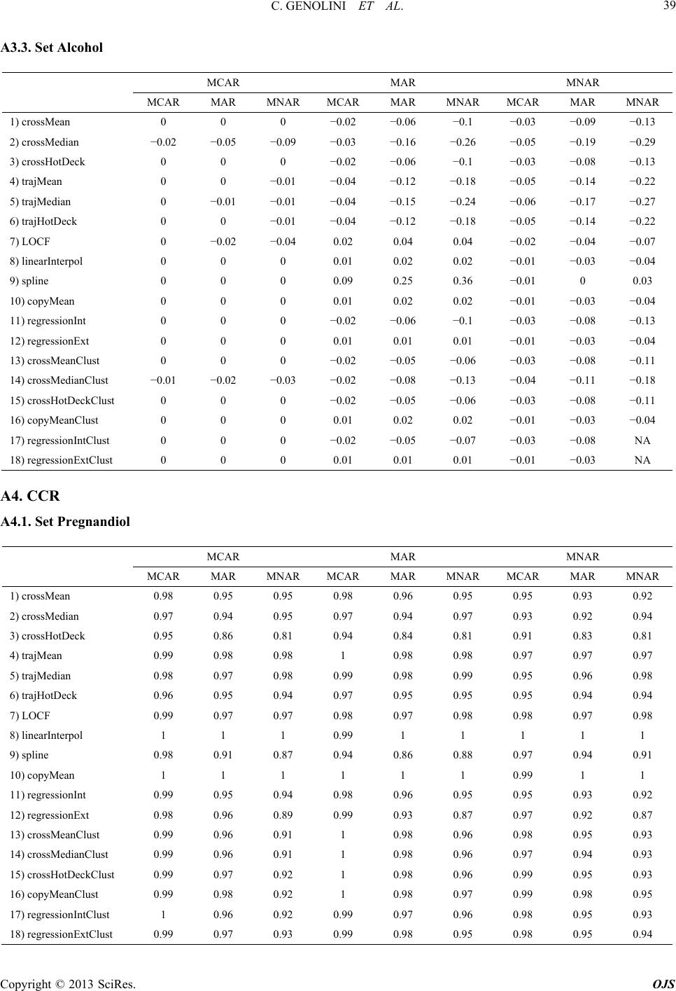. GENOLINI ET AL. 39

A3.3. Set Alcohol

MCAR MAR MNAR

MCAR MAR MNAR MCAR MAR MNAR MCAR MAR MNAR

1) crossMean 0 0 0 −0.02 −0.06 −0.1 −0.03 −0.09 −0.13

2) crossMedian −0.02 −0.05 −0.09 −0.03 −0.16 −0.26 −0.05 −0.19 −0.29

3) crossHotDeck 0 0 0 −0.02 −0.06 −0.1 −0.03 −0.08 −0.13

4) trajMean 0 0 −0.01 −0.04 −0.12 −0.18 −0.05 −0.14 −0.22

5) trajMedian 0 −0.01 −0.01 −0.04 −0.15 −0.24 −0.06 −0.17 −0.27

6) trajHotDeck 0 0 −0.01 −0.04 −0.12 −0.18 −0.05 −0.14 −0.22

7) LOCF 0 −0.02 −0.04 0.02 0.04 0.04 −0.02 −0.04 −0.07

8) linearInterpol 0 0 0 0.01 0.02 0.02 −0.01 −0.03 −0.04

9) spline 0 0 0 0.09 0.25 0.36 −0.01 0 0.03

10) copyMean 0 0 0 0.01 0.02 0.02 −0.01 −0.03 −0.04

11) regressionInt 0 0 0 −0.02 −0.06 −0.1 −0.03 −0.08 −0.13

12) regressionExt 0 0 0 0.01 0.01 0.01 −0.01 −0.03 −0.04

13) crossMeanClust 0 0 0 −0.02 −0.05 −0.06 −0.03 −0.08 −0.11

14) crossMedianClust −0.01 −0.02 −0.03 −0.02 −0.08 −0.13 −0.04 −0.11 −0.18

15) crossHotDeckClust 0 0 0 −0.02 −0.05 −0.06 −0.03 −0.08 −0.11

16) copyMeanClust 0 0 0 0.01 0.02 0.02 −0.01 −0.03 −0.04

17) regressionIntClust 0 0 0 −0.02 −0.05 −0.07 −0.03 −0.08 NA

18) regressionExtClust 0 0 0 0.01 0.01 0.01 −0.01 −0.03 NA

A4. CCR

A4.1. Set Pregnandiol

MCAR MAR MNAR

MCAR MAR MNAR MCAR MAR MNAR MCAR MAR MNAR

1) crossMean 0.98 0.95 0.95 0.98 0.96 0.95 0.95 0.93 0.92

2) crossMedian 0.97 0.94 0.95 0.97 0.94 0.97 0.93 0.92 0.94

3) crossHotDeck 0.95 0.86 0.81 0.94 0.84 0.81 0.91 0.83 0.81

4) trajMean 0.99 0.98 0.98 1 0.98 0.98 0.97 0.97 0.97

5) trajMedian 0.98 0.97 0.98 0.99 0.98 0.99 0.95 0.96 0.98

6) trajHotDeck 0.96 0.95 0.94 0.97 0.95 0.95 0.95 0.94 0.94

7) LOCF 0.99 0.97 0.97 0.98 0.97 0.98 0.98 0.97 0.98

8) linearInterpol 1 1 1 0.99 1 1 1 1 1

9) spline 0.98 0.91 0.87 0.94 0.86 0.88 0.97 0.94 0.91

10) copyMean 1 1 1 1 1 1 0.99 1 1

11) regressionInt 0.99 0.95 0.94 0.98 0.96 0.95 0.95 0.93 0.92

12) regressionExt 0.98 0.96 0.89 0.99 0.93 0.87 0.97 0.92 0.87

13) crossMeanClust 0.99 0.96 0.91 1 0.98 0.96 0.98 0.95 0.93

14) crossMedianClust 0.99 0.96 0.91 1 0.98 0.96 0.97 0.94 0.93

15) crossHotDeckClust 0.99 0.97 0.92 1 0.98 0.96 0.99 0.95 0.93

16) copyMeanClust 0.99 0.98 0.92 1 0.98 0.97 0.99 0.98 0.95

17) regressionIntClust 1 0.96 0.92 0.99 0.97 0.96 0.98 0.95 0.93

18) regressionExtClust 0.99 0.97 0.93 0.99 0.98 0.95 0.98 0.95 0.94

C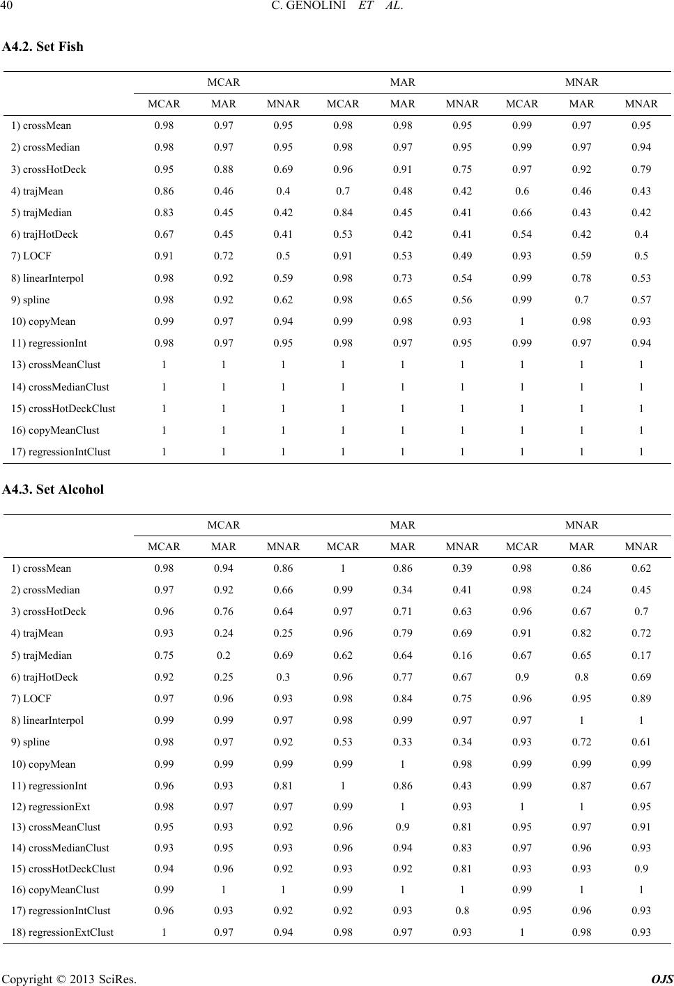. GENOLINI ET AL.

A4.2. Set Fish

MCAR MAR MNAR

MCAR MAR MNAR MCAR MAR MNAR MCAR MAR MNAR

1) crossMean 0.98 0.97 0.95 0.98 0.98 0.95 0.99 0.97 0.95

2) crossMedian 0.98 0.97 0.95 0.98 0.97 0.95 0.99 0.97 0.94

3) crossHotDeck 0.95 0.88 0.69 0.96 0.91 0.75 0.97 0.92 0.79

4) trajMean 0.86 0.46 0.4 0.7 0.48 0.42 0.6 0.46 0.43

5) trajMedian 0.83 0.45 0.42 0.84 0.45 0.41 0.66 0.43 0.42

6) trajHotDeck 0.67 0.45 0.41 0.53 0.42 0.41 0.54 0.42 0.4

7) LOCF 0.91 0.72 0.5 0.91 0.53 0.49 0.93 0.59 0.5

8) linearInterpol 0.98 0.92 0.59 0.98 0.73 0.54 0.99 0.78 0.53

9) spline 0.98 0.92 0.62 0.98 0.65 0.56 0.99 0.7 0.57

10) copyMean 0.99 0.97 0.94 0.99 0.98 0.93 1 0.98 0.93

11) regressionInt 0.98 0.97 0.95 0.98 0.97 0.95 0.99 0.97 0.94

13) crossMeanClust 1 1 1 1 1 1 1 1 1

14) crossMedianClust 1 1 1 1 1 1 1 1 1

15) crossHotDeckClust 1 1 1 1 1 1 1 1 1

16) copyMeanClust 1 1 1 1 1 1 1 1 1

17) regressionIntClust 1 1 1 1 1 1 1 1 1

A4.3. Set Alcohol

MCAR MAR MNAR

MCAR MAR MNAR MCAR MAR MNAR MCAR MAR MNAR

1) crossMean 0.98 0.94 0.86 1 0.86 0.39 0.98 0.86 0.62

2) crossMedian 0.97 0.92 0.66 0.99 0.34 0.41 0.98 0.24 0.45

3) crossHotDeck 0.96 0.76 0.64 0.97 0.71 0.63 0.96 0.67 0.7

4) trajMean 0.93 0.24 0.25 0.96 0.79 0.69 0.91 0.82 0.72

5) trajMedian 0.75 0.2 0.69 0.62 0.64 0.16 0.67 0.65 0.17

6) trajHotDeck 0.92 0.25 0.3 0.96 0.77 0.67 0.9 0.8 0.69

7) LOCF 0.97 0.96 0.93 0.98 0.84 0.75 0.96 0.95 0.89

8) linearInterpol 0.99 0.99 0.97 0.98 0.99 0.97 0.97 1 1

9) spline 0.98 0.97 0.92 0.53 0.33 0.34 0.93 0.72 0.61

10) copyMean 0.99 0.99 0.99 0.99 1 0.98 0.99 0.99 0.99

11) regressionInt 0.96 0.93 0.81 1 0.86 0.43 0.99 0.87 0.67

12) regressionExt 0.98 0.97 0.97 0.99 1 0.93 1 1 0.95

13) crossMeanClust 0.95 0.93 0.92 0.96 0.9 0.81 0.95 0.97 0.91

14) crossMedianClust 0.93 0.95 0.93 0.96 0.94 0.83 0.97 0.96 0.93

15) crossHotDeckClust 0.94 0.96 0.92 0.93 0.92 0.81 0.93 0.93 0.9

16) copyMeanClust 0.99 1 1 0.99 1 1 0.99 1 1

17) regressionIntClust 0.96 0.93 0.92 0.92 0.93 0.8 0.95 0.96 0.93

18) regressionExtClust 1 0.97 0.94 0.98 0.97 0.93 1 0.98 0.93
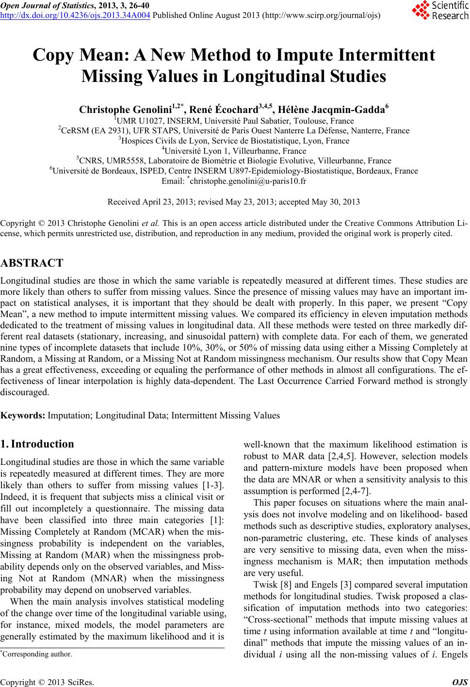