Open Journal of Statistics, 2013, 3, 16-25
http://dx.doi.org/10.4236/ojs.2013.34A003 Published Online August 2013 (http://www.scirp.org/journal/ojs)
Log-Link Regression Models for Ordinal Responses
Christopher L. Blizzard1, Stephen J. Quinn2, Jana D. Canary1, David W. Hosmer3
1Menzies Research Institute Tasmania, University of Tasmania, Hobart, Australia
2Flinders Clinical Effectiveness, Flinders University, Adelaide, Australia
3Department of Public Health, University of Massachusetts, Amherst, USA
Received June 9, 2013; revised July 9, 2013; accepted July 16, 2013
Copyright © 2013 Christopher L. Blizzard et al. This is an open access article distributed under the Creative Commons Attribution
License, which permits unrestricted use, distribution, and reproduction in any medium, provided the original work is properly cited.
ABSTRACT
The adjacent-categories, continuation-ratio and proportional odds logit-link regression models provide useful extensions
of the multinomial logistic model to ordinal response data. We propose fitting these models with a logarithmic link to
allow estimation of different forms of the risk ratio. Each of the resulting ordinal response log-link models is a con-
strained version of the log multinomial model, the log-link counterpart of the multinomial logistic model. These models
can be estimated using software that allows the user to specify the log likelihood as the objective function to be maxi-
mized and to impose constraints on the parameter estimates. In example data with a dichotomous covariate, the uncon-
strained models produced valid coefficient estimates and standard errors, and the constrained models produced plausible
results. Models with a single continuous covariate performed well in data simulations, with low bias and mean squared
error on average and appropriate confidence interval coverage in admissible solutions. In an application to real data,
practical aspects of the fitting of the models are investigated. We conclude that it is feasible to obtain adjusted estimates
of the risk ratio for ordinal outcome data.
Keywords: Ordinal; Risk Ratio; Multinomial Likelihood; Logarithmic Link; Log Multinomial Regression; Adjacent
Categories; Continuation-Ratio; Proportional Odds; Ordinal Logistic Regression
1. Introduction
Several logit-link regression models have been proposed
to deal with ordered categorical response data. Three of
these are the adjacent categories model [1], the continua-
tion-ratio model [2], and the cumulative odds model [3].
The last is referred to also as the proportional odds model
[4]. The basis of each of these models is the discrete
choice model [5] for nominal categorical outcomes that
are also termed the multinomial logistic regression model
[6].
The purpose of this paper is to investigate the practi-
cality of fitting the ordinal models with a logarithmic link
in place of the logit link. We refer to the resulting models
as the adjacent categories (AC) probability model, the
continuation-ratio (CR) probability model, and the pro-
portional probability (PP) model. Each is a constrained
form of the log multinomial model [7], the log-link
counterpart of the multinomial logistic model. The ordi-
nal log-link models make it possible to directly estimate
different but related forms of the risk ratio in prospective
studies and the prevalence ratio in cross-sectional studies,
overcoming thereby a limitation of logit-link models.
Epidemiological research is grounded largely in assess-
ment of average risk, and in that field the worth of the
odds ratio as a measure of effect has long been ques-
tioned [8,9] particularly for prospective [10] and cross-
sectional [11] data.
To describe the log-link models for ordinal data, we
have adapted specialist terminology used for ordinal lo-
gistic models. Several authors [6,12,13] have distin-
guished “forwards” and “backwards” versions of the CR
logit-link model, with the outcome categories taken in
reverse order in the “backwards” version. For propor-
tional odds models, O’Connell [14] distinguished bet-
ween an “ascending” version for lower-ordered catego-
ries versus higher categories, and a “descending” version
for higher-ordered categories versus lower categories. Ac-
cordingly, we distinguish “forwards-ascending” and “for-
wards-descending” versions of the AC probability model
and the PP model. The two versions of each model pro-
duce coefficients that differ both in sign and magnitude.
For the CR probability model, it is necessary to addition-
ally distinguish “backwards-ascending” and “backwards-
descending” versions because the four possible versions
each produce a different set of estimates. For brevity, we
C
opyright © 2013 SciRes. OJS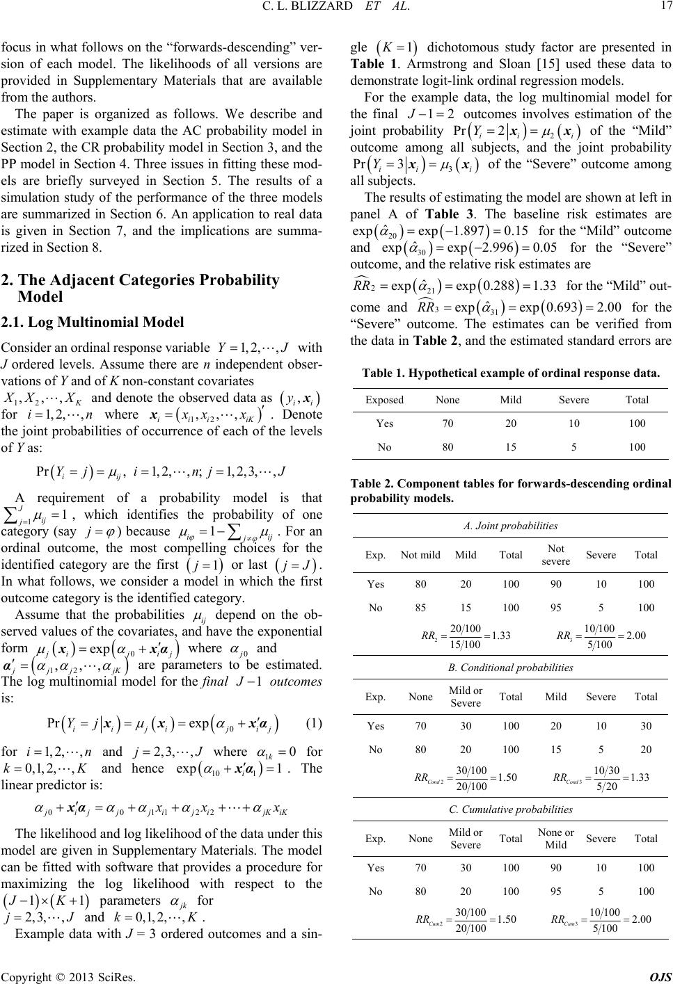

C. L. BLIZZARD ET AL. 17
focus in what follows on the “forwards-descending” ver-
sion of each model. The likelihoods of all versions are
provided in Supplementary Materials that are available
from the authors.
The paper is organized as follows. We describe and
estimate with example data the AC probability model in
Section 2, the CR probability model in Section 3, and the
PP model in Section 4. Three issues in fitting these mod-
els are briefly surveyed in Section 5. The results of a
simulation study of the performance of the three models
are summarized in Section 6. An application to real data
is given in Section 7, and the implications are summa-
rized in Section 8.
2. The Adjacent Categories Probability
Model
2.1. Log Multinomial Model
Consider an ordinal response variable with
J ordered levels. Assume there are n independent obser-
vations of Y and of K non-constant covariates
12
1, 2,,YJ
,,,
K
X
XX and denote the observed data as


,
ii
xy

,,, for where 12iii iK 1, 2,,in
x
xx

x. Denote
the joint probabilities of occurrence of each of the levels
of Y as:

Pr,1,2,,; 1,2,3,,
iij
Yj injJ   
A requirement of a probability model is that
1j, which identifies the probability of one
category (say
1
J
ij
 
j

) because j
j

1
ii

. For an
ordinal outcome, the most compelling choices for the
identified category are the first or last



1j


jJ

.
In what follows, we consider a model in which the first
outcome category is the identified category.
Assume that the probabilities ij

depend on the ob-
served values of the covariates, and have the exponential
form
 
0
exp
j
ij


xxα
ij
where 0
j

and

12
,,,
j
jj jK
are parameters to be estimated.
The log multinomial model for the final


α
1
J
 outcomes
is:



0
Pr exp
iiji ji
Yj 

 xx xαj (1)
for and where
1, 2,,in2,3, ,jJ10
k


for
and hence . The
linear predictor is:
0,1,2,,kK

10 i
 
xα

11

exp 
001122
j
ijjjij ijKiK
x
xx

 

 xα
The likelihood and log likelihood of the data under this
model are given in Supplementary Materials. The model
can be fitted with software that provides a procedure for
maximizing the log likelihood with respect to the
parameters

1JK 

1
j
k

for
and .
2, 3,,jJ0,1,2,,kK
Example data with J = 3 ordered outcomes and a sin-
gle


1K

dichotomous study factor are presented in
Table 1. Armstrong and Sloan [15] used these data to
demonstrate logit-link ordinal regression models.
For the example data, the log multinomial model for
the final 12J

 outcomes involves estimation of the
joint probability



2
Pr 2Y  xx
ii i
of the “Mild”
outcome among all subjects, and the joint probability




3
Pr 3
ii
Y  xi x of the “Severe” outcome among
all subjects.
The results of estimating the model are shown at left in
panel A of Table 3. The baseline risk estimates are




20
ˆ expexp1.8970.15    for the “Mild” outcome
and




30
ˆ expexp2.996   0.05  for the “Severe”
outcome, and the relative risk estimates are

 
221
ˆ
expexp 0.2881.33RR
   for the “Mild” out-
come and

 
331
ˆ
expexp 0.6932.00RR
   for the
“Severe” outcome. The estimates can be verified from
the data in Table 2, and the estimated standard errors are
Table 1. Hypothetical example of ordinal response data.
Exposed None Mild Severe Total
Yes 70 20 10 100
No 80 15 5 100
Table 2. Component tables for forw ards-descending ordinal
probability models.
A. Joint probabilities
Exp. Not mildMild Total Not
severe Severe Total
Yes 80 20 100 90 10 100
No 85 15 100 95 5 100
2
20 1001.33
15 100
RR  3
10 1002.00
5100
RR 
B. Conditional probabilities
Exp. NoneMild or
Severe Total Mild SevereTotal
Yes 70 30 100 20 10 30
No 80 20 100 15 5 20
2
30 1001.50
20 100
Cond
RR  3
10 301.33
520
Cond
RR 
C. Cumulative probabilities
Exp. NoneMild or
Severe Total None or Mild Severe Total
Yes 70 30 100 90 10 100
No 80 20 100 95 5 100
2
30 1001.50
20 100
Cum
RR  3
10 1002.00
5100
Cum
RR 

C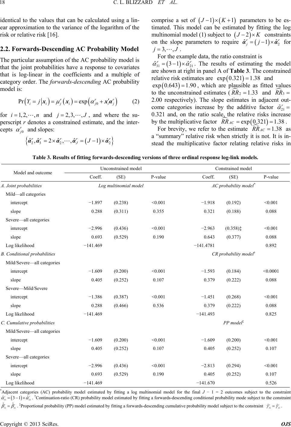. L. BLIZZARD ET AL.
18
comprise a set of




1JK
identical to the values that can be calculated using a lin-
ear approximation to the variance of the logarithm of the
risk or relative risk [16].
1

 parameters to be es-
timated. This model can be estimated by fitting the log
multinomial model (1) subject to

2
J
K
ˆjj
constraints
on the slope parameters to require for

2
ˆ
1
rr
αα
3, ,jJ

. 2.2. Forwards-Descending AC Probability Model
For the example data, the ratio constraint is


31 21
ˆˆ 31
r
The particular assumption of the AC probability model is
that the joint probabilities have a response to covariates
that is log-linear in the coefficients and a multiple of
category order. The forwards-descending AC probability
model is:
r

  . The results of estimating the model
are shown at right in panel A of Table 3. The constrained
relative risk estimates are and

exp 0.3211.38


exp 0.6431.90, which are plausible as fitted values
to the unconstrained estimates (

21.33RR and

3 RR

2.00 respectively). The slope estimates in adjacent out-
come categories increase by the additive factor 21 ˆr 

0.321 and, on the ratio scale, the relative risks increase
by the multiplicative factor


exp 0.321 AC RR 1.38 .



0
Pr exp
rr
iiji ji
Yj 

 xx xα

r
j
J
(2)
for and , and where the su-
perscript r denotes a constrained estimate, and the inter-
cepts
1, 2,,in
0
r
2,3, ,j
j

and slopes:

1.38 AC RR 
For brevity, we refer to the estimate


23 22
ˆˆˆˆ ˆ
,2,, 1
r
JJααα αα

as
a “summary” relative risk when strictly it is not. It is in-
stead the multiplicative factor relating relative risks in
rrr r
Table 3. Results of fitting forwards-descending versions of three ordinal response log-link models.
Unconstrained model Constrained model
Model and outcome Coeff. (SE) P-value Coeff. (SE) P-value
A. Joint probabilities Log multinomial model AC probability model*
Mild—all categories
intercept −1.897(0.238) <0.001 −1.918(0.192) <0.001
slope 0.288(0.311) 0.355 0.321(0.188) 0.088
Severe—all categories
intercept −2.996(0.436) <0.001 −2.963(0.358)‡ <0.001
slope 0.693(0.529) 0.190 0.643(0.377) 0.088
Log likelihood −141.469 −141.4781 0.892
B. Conditional probabilities CR probability model†
Mild/Severe—all categories
intercept −1.609(0.200) <0.001 −1.593(0.184) <0.0001
slope 0.405(0.252) 0.107 0.379(0.222) 0.088
Severe—Mild/Severe
intercept −1.386(0.387) <0.001 −1.451(0.268) <0.001
slope 0.288(0.466) 0.536 0.379(0.222) 0.088
Log likelihood −141.469 −141.493 0.825
C. Cumulative probabilities PP model‡
Mild/Severe—all categories
intercept −1.609(0.200) <0.001 −1.609(0.200) <0.001
slope 0.405(0.252) 0.107 0.405(0.252) 0.107
Severe—all categories
intercept −2.996(0.436) <0.001 −2.813(0.294) <0.001
slope 0.693(0.529) 0.190 0.405(0.252) 0.107
Log likelihood −141.469 −141.670 0.526
*Adjacent categories (AC) probability model estimated by fitting a log multinomial model for the final J − 1 = 2 outcomes subject to the constraint

31 21
ˆ 31
c
ˆ
c

 
31 21
ˆˆ
cc
. †Continuation-ratio (CR) probability model estimated by fitting a forwards-descending conditional probability mode subject to the constraint

. ‡Proportional probability (PP) model estimated by fitting a forwards-descending cumulative probability model subject to the constraint 31 21
ˆˆ
cc


.

C. L. BLIZZARD ET AL. 19
adjacent categories. It does not represent a common rela-
tive risk of advancing to the higher of adjacent categories,
because that would require
  
112
rrr r
j
ijijij i
 

xx xx
J
J
for when, in general, these ratios are un-
equal and differ for each covariate holding.
3, ,j
2.3. Assessment of Loss of Model Fit
Three equivalent large-sample methods [17] are available
to assess whether the constraints result in significant loss
of model fit. Each has an asymptotic distribution that is
chi-squared with degrees of freedom equal to the number
of additional constraints imposed. Firstly, a test may be
based on the likelihood ratio criterion [18]. Secondly, a
test may be based on the efficient scores criterion [19].
Thirdly, a test may be based on the criterion proposed by
Wald [20]. For a fully-constrained AC probability model
in which the constraint is applied to each covariate, the
null hypothesis for these tests is that
for . It is possible to apply the constraints
to a subset of the covariates in a partially-constrained
model [21], and to test a composite hypothesis. Readers
are referred to Rao [17] for details.

2
1
jjαα
2, 3,,j
For the example data, the AC probability model with
log likelihood −141.478 is a constrained version of a log
multinomial model with log likelihood –141.469. A like-
lihood ratio test with test statistic
and one de-
gree of freedom gives

2 141.478141.4690.019
o
G  




2
Pr1 0.019  

0.891. The
score and Wald statistics are identical in the first four
decimal places. The results suggest that the effect of ex-
posure has been summarized into a single relative risk
without significant loss of model fit.
3. The Continuation-Ratio Probability Mod-
el
3.1. Forwards-Descending Conditional Model
Consider ordinal outcome data arising from a hierarchi-
cal sequence of binary events in which the probability at
each stage is conditional on having reached that stage.
McCullagh and Nelder [22] provide an example of in-
semination of milch cows, and propose a model of the
probability of impregnation of a cow at the attempt
after unsuccessful attempts. This is the prob-
ability of terminating at the stage conditional on
having reached that stage. O’Connell [14] provides an
example of childhood proficiency in literacy in which
mastery of any level of literacy requires mastery of all
previous levels, and interest lies in the probability of
success at a higher level. This is the probability of ad-
vancing beyond the
th
j

1j

th
j

1
s
t
j stage conditional on hav-
ing reached that stage. Denote that probability as:


Pr1,1, 2,,;2,3,,
ii ij
YjYji njJ  
Assume that the conditional probabilities ij

depend
also upon the observed values of the covariates, and have
the exponential form


exp

0
j
i
 xx
j
  
ij
β
where
0
j

and jjjjK are parameters to be
estimated. The forwards-descending conditional prob-
ability model is:

12
,,, 

  β




0
Pr 1, exp
ii ijiji
YjYj 
j

 xx x
β
(3)
for 1, 2,,in

 and 2,3,,jJ

 where 10
k


for
0,1, 2,,kK

 and hence . The
linear predictor is:

10 i
 xβ

11exp

001122
j
ijjjij ijKiK
x
xx



 xβ
The likelihood and log likelihood of the data under this
model are given in Supplementary Materials. The model
can be fitted with software that provides a procedure for
maximising the log likelihood with respect to its




1JK1

 parameters
j
k

for and 2,3, ,jJ
0,1, 2,,kK

. An alternative approach to fitting the
model is also described in Supplementary Materials.
For the example data, the forwards-descending condi-
tional probability model involves estimating the condi-
tional probability

 
2
Pr21,
iii i
of a
“Mild” or “Severe” outcomes among all subjects, and the
conditional probability
YY   xx




3
Pr3 2,
ii ii
of
the “Severe” outcome among subjects with a “Mild” or
“Severe” outcome. The component tables for the model
are shown in panel B of Table 2.
YY   xx
The results of estimating the model are shown at left in
panel B of Table 3. The relative conditional risk esti-
mates are

 2exp0.4051.50 Cond
RR  and


exp 0.2881.33 3Cond RR . Those estimates and their
estimated standard errors can be verified from the data in
Table 2.
3.2. Forwards-Descending CR Probability Model
The particular assumption of CR probability models is
that the conditional probabilities have a response to co-
variates that is independent of the outcome category and
log-linear in the coefficients.
The forwards-descending CR probability model is:




0
Pr 1, exp
cc
ii ijijij
YjYj 
c

 xx x
β
(4)
for 1, 2,,in

 and 2,3,,jJ

 where the super-
script denotes a constrained estimate, and intercepts
0
c
c
j

and common slope coefficients 23
cc c
J
ββ
β

comprise a set of




11JK


parameters to be es-
timated of which only


12J

are unique. This
model can be estimated by fitting the conditional prob-
ability model (3) subject to


2
J
K constraints on

C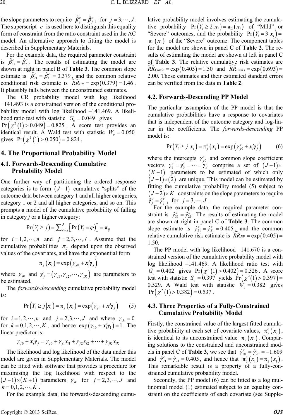. L. BLIZZARD ET AL.
20
the slope parameters to require 1
ˆˆ
cc
j
j
β
β
for 3, ,jJ

.
The superscript is used here to distinguish this equality
form of constraint from the ratio constraint used in the AC
model. An alternative approach to fitting the model is
described in Supplementary Materials.
c
For the example data, the required parameter constraint
is 31 21
ˆˆ
cc

 . The results of estimating the model are
shown at right in panel B of Table 3. The common slope
estimate is 21 31, and the common relative
conditional risk estimate is
ˆˆ
0.379
cc
 


379 1.46
0.050
o
W
exp
CR
RR
0.049
o
0..
It plausibly falls between the unconstrained estimates.
The CR probability model with log likelihood
−141.493 is a constrained version of the conditional pro-
bability model with log likelihood –141.469. A likeli-
hood ratio test with statistic gives
. A score test provides an
identical result. A Wald test with statistic
G


2
Pr1 00.825  .049

gives .


2
Pr1 0.050  0.824


Pr
ii
Y 
 

3,, J
4. The Proportional Probability Model
4.1. Forwards-Descending Cumulative
Probability Model
One further way of partitioning the ordered response
categories is to form cumulative “splits” of the
outcome data between category 1 and all higher categories,
category 1 or 2 and all higher categories, and so on. This
prompts a model of the cumulative probability of falling
in category j or a higher category:

1J
 
Pr π
J
j  
 
ij
Yj
for and . Assume that the
cumulative probabilities ij
1,2,,in2,j

depend upon the observed
values of the covariates, and have the exponential form



0
πexp
j
ij


 xx
ij
γ
where 0
j

and

12
,,

,
j
jj jK
 

γ are parameters to
be estimated.
The forwards-descending cumulative probability model
is:






0
Pr π
iij j
xxexp
i
 
,, J
ij

xγ
10 k
Yj (5)
for and and where 1, 2,,in2,3j


for , and hence . The
linear predictor is:
0,1, 2,k,K

i

 x

11γ 10
exp 
11200 2
j
ijjj ijijKiK
x
xx

xγ 
The likelihood and log likelihood of the data under this
model are given in Supplementary Materials. The model
can be fitted with software that provides a procedure for
maximising the log likelihood with respect to the




1JK 1 parameters
j
k

for and
.
2, 3,,jJ
0,1, 2,,kK
For the example data, the forwards-descending cumu-
lative probability model involves estimating the cumula-
tive probability




2
Pr 2π
ii i
of “Mild” or
“Severe” outcomes, and the probability
Yxx

Pr 3
ii
Y

x


3
πi x of the “Severe” outcome. The component tables
for the model are shown in panel C of Table 2. The re-
sults of estimating the model are shown at left in panel C
of Table 3. The relative cumulative risk estimates are


exp 0.4051.50 2Cum
R
R
and


3exp 0.693 Cum RR 
2.00. Those estimates and their estimated standard errors
can be verified from the data in Table 2.
4.2. Forwards-Descending PP Model
The particular assumption of the PP model is that the
cumulative probabilities have a response to covariates
that is independent of the outcome category and log-lin-
ear in the coefficients. The forwards-descending PP
model is:






0
Pr πexp
cc
iiji ji
Yj 

  xx x
c
j
γ
(6)
where the intercepts 0
c
j

and common slope coefficient
vectors 23
cc c
J

γγγ comprise a set of


1J




1K

parameters to be estimated of which only




21J are unique. This model can be estimated by
fitting the cumulative probability model (5) subject to


2
J
K


c constraints on the slope parameters to require
1
ˆˆ
c
j
j

γ
γ
for 3, ,jJ

.
For the example data, the required parameter con-
straint is 31 21
ˆˆ
cc

 . The results of estimating the model
are shown at right in panel C of Table 3. The common
slope estimate is 2131, and the common
relative cumulative risk estimate is
ˆˆ0.405
cc
 


exp 0.405
PP
R
R
1.50.
The PP model with log likelihood –141.670 is a con-
strained version of the cumulative probability model with
log likelihood –141.469. A likelihood ratio test with
0.402
o
G

gives




2
Pr1 0.4020.526  
0.397
o
. A score
test with statistic S

yields



0.397
2
2
Pr 1 
0.38
o
W 0.529. A Wald test with statistic gives




2
Pr 1  0.3820.537.
4.3. Three Properties of a Fully-Constrained
Cumulative Probability Model
Firstly, the constrained value of the largest fitted cumula-
tive probability at each set of covariate values,


2
πci x
1.609
,
is identical to its unconstrained value . Compar-
ing solutions to the constrained and unconstrained mod-
els in panel C of Table 3, we see that
and 21 21, and hence that

2
πi x
20 20
ˆˆ
c



ˆˆ0.405
c
 



21 21
ππ
c
x
x.
This remarkable result is a property of a fully-con-
strained cumulative probability model.
Secondly, the PP model (6) can be fitted as a log mul-
tinomial model (1) estimated subject to an equality con-
straint on the coefficients of each covariate (see Supple-

C. L. BLIZZARD ET AL. 21
mentary Materials). Hence the common slope estimate
21 31 from the fully constrained cumulative
probability model can be seen as a summary estimate for
the unconstrained slope estimates 21
ˆˆ0.405
cc
 
ˆ0.288

 from the
log multinomial model. The PP model forces these joint
probabilities to be equal.
Thirdly, in a fully-constrained model, the fitted prob-
abilities

ˆ πc
j
i
x

are proportional in the sense that







12 1
11
ˆˆˆ ˆ ππ ππ
cc cc
jijij ij i 
xxxx
2
and








112
1
ˆˆˆˆ
πππ π
ccc c
jij ijij i 
xxx 2
1 
x
J

To confirm that the three ordinal log-link regression
for where and denote distinct
covariate holdings. These ratio equalities justify the de-
scription of the fully-constrained cumulative probability
model as a proportional probability (PP) model.
3, ,j

1
i
x

2
i
x
5. Issues in Fitting the Models
5.1. Starting Values
A careful choice of starting values is required for the
cumulative probability models. This is a consequence of
the need to evaluate terms of the form

in the log likelihood. As starting
values we use the estimates from the common-slopes log
multinomial model, with intercept values derived from
the recursive relation given previously.
 
1
ln ππ
jij i
 

xx
5.2. Non-Admissable Solutions
Solutions to a probability model are not admissible if any
of the fitted probabilities exceed unity and if the sum of
the fitted probabilities exceeds unity. The functional
form of the three ordinal models does not constrain the
fitted probabilities to take admissible values, and hence
non-admissible solutions can occur in the extremes of
covariate space if the model-based probabilities are very
high.
5.3. Non-Convergence
The log likelihoods for each model contain terms that
cannot be evaluated if the fitted values of the probabili-
ties, or their sums in the AC model, reach or exceed unity.
This may prevent convergence to a solution. For model-
based simulated data, the simple expedient of requiring
evaluation of a term in the log likelihood only if its coef-
ficient is non-zero eliminates almost all problems with
convergence. Converged but non-admissible solutions
are produced instead. We take advantage of this to study
non-admissible solutions in the next section.
6. Simulation Study
models produce estimates that match their theoretical
values on average and without excessive variation, and
with estimated standard errors that provide appropriate
confidence interval coverage, we repeatedly generated
data from each probability model and fitted the ordinal
models to each dataset. The simulations involved a single


1K

uniformly-distributed covariate X and a re-
ariable Y having 3J ordered levels with sponse v


Pr20 0.12Yx ,

Pr0 0.04Yx and 3






Pr Yj 1 1.10x YjxPr

 . We d-
ples of size
rew sam
200n

and , an
of repl to pro
he three ordinal log-link regression models
pr
500nd with an ade-
quate number icationsduce at least 10,000
admissible solutions and at least 1000 non-admissible
solutions in two settings. The settings used and methods
of generating the data are described in the Supplementary
Materials. The results are presented there as average
percent relative bias, average percent mean squared error
and average 95 percent confidence interval coverage.
Additionally, the results of likelihood ratio, score and
Wald tests of the constraint imposed in each model were
recorded.
Each of t
oduced estimates with minimal bias and mean squared
error on average, and with 95 percent confidence interval
coverage that was close to the nominal 95 percent. The
summary model fit statistics were similar for each model,
and the minor differences did not impart a clear advan-
tage for any single model. Type 1 error rates were close
to 5 percent but, particularly for the CR probability mod-
el, with a tendency to reject slightly too often. At larger
values of the uniform covariate, for which the theoretical
values from three probability models are most different,
power to reject an incorrect model was moder- ate for
each of the AC probability model and the PP model, and
higher for the CR probability model. Bias and mean
squared error were smaller, error rates on average were
closer to 5 percent, and power in each setting was greater,
in the larger datasets


500n than in the smaller da-
tasets


200n.
The comprecedingments refer to solutions for which
th
7. Application to Real Data
on 189 births to
e fitted values are admissible for a probability model. In
non-admissible solutions that were deliberately engi-
neered by allowing the uniform covariate to take large
values, model fit was less satisfactory because bias was
relatively high and confidence interval coverage was
greatly reduced, and the tendency for each model to reject
too often a correctly fitted model was more pronounced.
The dataset consists of information
women seen in the obstetrics clinic at Baystate Medical
Center in Springfield, Massachusetts. Hosmer and Le-
meshow [6] used these data to demonstrate ordinal logit-
link regression models. The ordered outcome consists of

C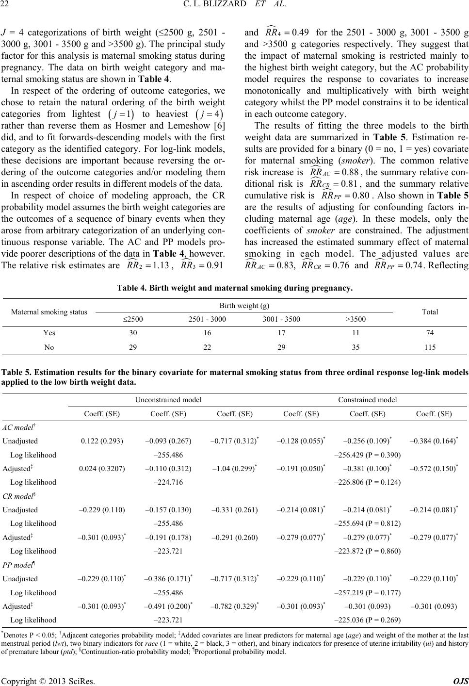. L. BLIZZARD ET AL.
22
tegories, we
ch
J = 4 categorizations of birth weight (2500 g, 2501 -
3000 g, 3001 - 3500 g and >3500 g). The principal study
factor for this analysis is maternal smoking status during
pregnancy. The data on birth weight category and ma-
ternal smoking status are shown in Table 4.
In respect of the ordering of outcome ca
ose to retain the natural ordering of the birth weight
categories from lightest

1j

to heaviest


4j

rather than reverse them aser and Lemesh
did, and to fit forwards-descending models with the first
category as the identified category. For log-link models,
these decisions are important because reversing the or-
dering of the outcome categories and/or modeling them
in ascending order results in different models of the data.
In respect of choice of modeling approach, the CR
Hosmow [6]
probability model assumes the birth weight categories are
the outcomes of a sequence of binary events when they
arose from arbitrary categorization of an underlying con-
tinuous response variable. The AC and PP models pro-
vide poorer descriptions of the data in Table 4, however.
The relative risk estimates are

21.13RR,

30.91RR 
and

40.49RR  for the 2501 - 3000 g, 3001 - 3500 g
and >3500 g categories respectively. They suggest that
the impact of maternal smoking is restricted mainly to
the highest birth weight category, but the AC probability
model requires the response to covariates to increase
monotonically and multiplicatively with birth weight
category whilst the PP model constrains it to be identical
in each outcome category.
The results of fitting the three models to the birth
weight data are summarized in Table 5. Estimation re-
sults are provided for a binary (0 = no, 1 = yes) covariate
for maternal smoking (smoker). The common relative
risk increase is

0.88 AC RR , the summary relative con-
ditional risk is

0.81 CR RR , and the summary relative
cumulative risk is

0. PP RR 80. Also shown in Tabl e 5
are the results of adjusting for confounding factors in-
cluding maternal age (age). In these models, only the
coefficients of smoker are constrained. The adjustment
has increased the estimated summary effect of maternal
smoking in each model. The adjusted values are


and

0.74 PP RR . Reflecting 0.83 AC RR , RR 0.76 CR 
Table 4. Birth weight and maternal smoking during pregnanc y.
Birth weight (g)
Maternal smoking status 2500 2501 - 301 - 3500 >3500 Total
00 300
Yes 74 30 16 17 11
No 29 22 29 35 115
able 5. Estimation results for the binary covariate for maternal smoking status from three ordinal response log-link models
ained model Constrained model
T
applied to the low birth weight data.
Unconstr
Coeff. (SE) Coeff. (SE) Coeff. (SE) Coeff. (SE) Coeff. (SE) Coeff. (SE)
AC model†
Unadjusted 0.122 (.293) –0.093.267) –0.717 .312)* –0.128 .055)* –0.256 .109)* –0.384 .164)*
ood –2)
A0.024 (0.3207) –0.) –1.04 (0.299)* –0.191 (0.050)* –0.572 (0.150)*
ihood –2)
C
–0.229.110) –0.157.130) –0.331.261) –0.214 (.081)* –0.214 .081)* –0.214 .081)*
ood –2)
A–0.301 (0.093)* –0.) –0.291 (0.260) –0.279 (0.077)* –0.279 (0.077)*
ihood –2)
PP
–0.229 .110)* –0.386 .171)* –0.717 .312)* –0.229 .110)* –0.229 .110)* –0.229 .110)*
ood –2)
A–0.301 (0.093)* –0.)* –0.782 (0.329)* –0.301 (0.093)* –0.301 (0.093)
ihood –29)
0 (0(0(0 (0 (0
Log likelih–255.486 56.429 (P = 0.390
djusted‡ 110 (0.312–0.381 (0.100)*
Log likel–224.716 26.806 (P = 0.124
R model§
Unadjusted (0 (0 (00(0 (0
Log likelih–255.486 55.694 (P = 0.812
djusted‡ 191 (0.178–0.279 (0.077)*
Log likel–223.721 23.872 (P = 0.860
model¶
Unadjusted (0 (0 (0 (0 (0 (0
Log likelih–255.486 57.219 (P = 0.177
djusted‡ 491 (0.200–0.301 (0.093)
Log likel–223.721 25.036 (P = 0.26
*DAdjacent categories probabilityded covariates are linear predictors for maternal the mother at the last
enotes P < 0.05; † model; ‡Adage (age) and weight of
menstrual period (lwt), two binary indicators for race (1 = white, 2 = black, 3 = other), and binary indicators for presence of uterine irritability (ui) and history
of premature labour (ptd); §Continuation-ratio probability model; ¶Proportional probability model.

C. L. BLIZZARD ET AL. 23
the pronounced impact of maternal smoking in the high- advantage of doing so in simulated data is that the esti-
est birth weight category, the AC probability model es-
timate is less extreme that those of the CR model, and the
CR probability model estimate is less extreme than that
of the PP model. To simplify matters for demonstration
purposes, non-linearity in the scale of the continuous
covariates (particularly age) and statistical interaction
between covariates (including between smoker and age)
have been ignored. The resultant models had 6 or more
covariates including continuous variables, and produced
converged and admissible solutions. Non-convergence
was an occasional problem only, and occurred with very
complex models that involved higher-powered polyno-
mials of continuous variables and/or product terms for
statistical interaction.
The likelihood ratio tests reveal that the constraints
imposed to produce the summary estimates have resulted
in substantially greater loss of model fit for the AC and
PP models than for the CR model. If the subset

189n of data analyzed here is representative of all
dted in the birth weight study, the loss of model
fit would be statistically significant if the full dataset was
two (AC probability model), three (PP model) or 20 (CR
probability model) times larger in size.
8. Discussion
ata collec
In this paper, we proposed log-link alternatives to three
logistic regression models for ordinal data, and demon-
strated that it is possible to estimate these models with
software that allows the user to specify the log likelihood
as the objective function to be maximized and to impose
constraints on the parameter estimates. In example data
with a dichotomous covariate, the unconstrained models
produced relative risk estimates and estimated standard
errors that could be verified from the data, and the con-
strained estimates were credible approximations to the
unconstrained estimates. Models with a single continuous
covariate performed well in data simulations, with low
bias and mean squared error on average and appropriate
confidence interval coverage in admissible solutions.
Finally, the models were successfully fitted to a complex
real-world dataset with an ordinal outcome for which one
of the models provided a questionable theoretical expla-
nation but a superior practical description.
When the model-based probabilities were high, issues
in fitting the ordinal response log-link regression models
arose because the fitted probabilities are not restricted to
values less than unity. The estimation algorithm may fail
to converge or, if it does converge, the fitted values may
not be admissible for a probability model. It is possible to
write the algorithm in a manner that makes non-conver-
gence a rare occurrence in model-based simulated data
(less than 1 per 10,000 replications in our settings). The
mation algorithm converges to a non-admissible solution,
and this makes it feasible to study them. We found that
the estimated coefficients of the inadmissible solutions
had much greater bias on average, with estimated stan-
dard errors that were too small, and 95% confidence in-
terval coverage that was poorer in consequence. These
findings caution against relying on the results of non-
admissible solutions.
Each of the three ordinal response log-link models we
considered is a constrained version of the log multino-
mial model. The constraints impose a simple linear rela-
tion on the slope coefficients, and it is possible to test
whether the unconstrained model provides a better de-
scription of the data. We found that likelihood ratio,
score and Wald tests of the constraints each had close to
the correct type I error rates though they tended to be
slightly conservative. The power of tests for each model
to reject fits to data from any of the other ordinal re-
sponse log-link models increased with the size of the
maximum model-based probability, and was moderate to
high when the maximum model-based probability was
high.
In our estimation procedure, the user has flexibility to
place linear constraints on the coefficients of all, or some,
of the covariates. This makes it possible to fit “partially-
constrained” models in which the linear constraint is ap-
plied to a subset only of the explanatory variables [21].
In the analyses of the birth weight data, which focused on
the relationship between maternal smoking and birth
weight outcome, it served no purpose to place restrictions
on the other covariates, and to have constrained the coef-
ficients of maternal age would have significantly reduced
model fit.
The ordered birth weight data provided opportunity to
consider the choice of model, investigate the merits of
the fitted models, and probe the interpretation of the es-
timates in a real world setting. The modeling assump-
tions underlying the CR probability model were unten-
able for an outcome variable that arose from categoriza-
tion of birth weight, because the birth weight categories
did not truly arise as a hierarchy of binary events, but
otherwise there was much to recommend this model. The
constraint imposed in fitting the CR probability model
produced far less loss of model fit than the constraints
imposed in the other two models, and the summary esti-
mate—a 24 percent reduction in the conditional prob-
ability of higher birth weight outcomes for the infants of
mothers who smoked during pregnancy—was interpret-
able and plausible. Reasonably in the circumstances, it
fell between the estimates from the AC and PP models.
The limitations of this work should be kept in mind.
Firstly, the results are based on a simple data example for
a dichotomous covariate, a single set of data simulations

C. L. BLIZZARD ET AL.
24
for a continuous covariate and a response with just three
or
-
atio for ordinal outcome data. Particu-
del-based probabilities are high, how-
ard (CLB) provided by the National
ouncil of Australia.
Classifications Having Ordered Categories, Using Log-
Linear Models Log-Linear Models
for Odds,” Bio 1983, pp. 149-160.
dered levels, and an analysis of a single real-world
dataset in which issues with covariate scaling and statis-
tical interaction were ignored. Secondly, results have
been reported for the forwards-descending version of
each model without investigation of the merits of the
alternative versions. Thirdly, loss of model fit due to the
imposition of constraints on the coefficients was investi-
gated, but not the overall fit of the models. Fourthly, the
variance estimates are taken from the inverse of the ob-
served information matrix without thorough investigation
of using the expected information matrix in its place, or
of using an “information sandwich” to provide robust-
ness to model misspecification. The non-robust estimator
based on observed information provided confidence in-
terval coverage for the ordinal response models that was
about right, however. Fifthly, we used results based on
maximum likelihood theory to compute Wald-type con-
fidence intervals when the functional form of the log-link
models does not satisfy theoretical assumptions about the
parameter space required for distributional theory. Sixthly,
our investigation of power was limited to a single type of
model misspecification. It ignored other forms of depar-
ture such as omitted covariates and an incorrect link
function, and other issues including sample size and
model complexity, that would be taken into account in a
more complete investigation. Finally, we omitted a thor-
ough comparison of the merits of “partially-constrained”
and “fully-constrained” models, and of models with
non-linear constraints [21]. These may be important in
practice as a means of improving model fit when a linear
constraint applied across some covariates is untenable.
9. Conclusion
The three ordinal response log-link models offer a prac-
tical solution to the problem of obtaining adjusted esti
mates of the risk r
larly when the mo
ever, the models must be used with some care and atten-
tion to detail.
10. Acknowledgements
This work was funded by a project grant and Career De-
velopment Aw
Health and Medical Research C
REFERENCES
[1] L. A. Goodman. “The Analysis of Dependence in Cross-
for Frequencies and
metrics, Vol. 39, No. 1,
doi:10.2307/2530815
[2] S. E. Fienberg, “The Analysis of Cross-Classified Data,”
2nd Edition, MIT Press, Cambridge, 1980.
[3] S. H. Walker and D. B. Duncan, “Estimation of the Prob-
ability of an Event as a Function of Several Independent
Variables,” Biometrika, Vol. 54, No. 1, 1967, pp. 167-79.
ol. 42, No. 2,
[4] P. McCullough, “Regression Models for Ordinal Data,”
Journal of the Royal Statistical Society B, V
1980, pp. 109-142.
[5] D. McFadden, “Econometric Models for Probabilistic
Choice among Products,” Journal of Business, Vol. 53,
No. 3, 1980, pp. S13-S29. doi:10.1086/296093
[6] D. W. Hosmer and S. Lemeshow, “Applied Logistic Re-
gression,” 2nd Edition, Wiley, New York, 2000.
doi:10.1002/0471722146
[7] L. Blizzard and D. W. Hosmer, “Parameter Estimation
and Goodness-of-Fit in Log Binomial Regression,” Bio-
y, New
,” American Journal of Epidemiology, Vol.
. 23,
metrical Journal, Vol. 48, No. 6, 2006, pp. 5-22.
[8] O. S. Miettenen, “Theoretical Epidemiology,” Wile
York, 1985.
[9] S. Greenland, “Interpretation and Choice of Effect Meas-
ures in Epidemiologic Analysis,” American Journal of
Epidemiology, Vol. 125, No. 5, 1987, pp. 761-768.
[10] O. S. Miettenen and E. F. Cook, “Confounding: essence
and detection
114, No. 4, 1981, pp. 593-603.
[11] J. Lee, “Odds Ratio or Relative Risk for Cross-Sectional
Data?” International Journal of Epidemiology, Vol
No. 1, 1994, pp. 201-203. doi:10.1093/ije/23.1.201
[12] C. C. Clogg and E. S. Shihadeh, “Statistical Models for
Ordinal Variables,” Sage, Thousand Oaks, 1994.
[13] R. Bender and A. Benner, “Calculating Ordinal Regres-
sion Models in SAS and S-Plus,” Biometrical Journal,
Vol. 42, No. 6, 2000, pp. 677-699.
doi:10.1002/1521-4036(200010)42:6<677::AID-BIMJ67
7>3.0.CO;2-O
[14] A. A. O’Connell, “Logistic Regression Models for Ordi-
nal Response Variables,” Sage, Thousand Oaks, 2006.
[15] B. G. Armstrong and M. Sloan, “Ordinal Regressio
Models for Epidemiologic Data,” American Journal o
Epidemiology, V
n
f
ol. 129, No. 1, 1989, pp. 191-204.
rt
[16] D. Katz, J. Baptista, S. P. Azen and M. C. Pike, “Obtain-
ing Confidence Intervals for the Risk Ratio in Coho
Studies,” Biometrics, Vol. 34, 1978, pp. 469-474.
doi:10.2307/2530610.
[17] C. R. Rao, “Linear Statistical Inference and Its Applica-
, No.
240, 263-294.
lications to
tions,” 2nd Edition, Wiley, New York, 2002.
[18] J. Neyman and E. S. Pearson “On the Use and Interpreta-
tion of Certain Test Criteria,” Biometrika, Vol. 20
1/2, 3/4, 1928, pp. 175-
[19] C. R. Rao, “Large Sample Tests of Statistical Hypotheses
Concerning Several Parameters with App
Problems of Estimation,” Proceedings of the Cambridge
Philosophical Society, Vol. 44, No. 1, 1948, pp. 50-57.
doi:10.1017/S0305004100023987.
[20] A. Wald, “Tests of Statistical Hypotheses Concerning
Several Parameters When the Number of Observations Is
Large,” Transactions of the American Mathematical So-

C. L. BLIZZARD ET AL. 25
ciety, Vol. 54, No. 3, 1943, pp. 426-482.
doi:10.1090/S0002-9947-1943-0012401-3.
[21] B. Peterson and F. E. Harrrell, “Partial Proportional Odds
Models for Ordinal Response Variables,” Applied Statis-
tics, Vol. 39, No. 2, 1990, pp. 2005-2017.
doi:10.2307/2347760.
[22] P. McCullough and J. Nelder, “Generalized
els,” 2nd Edition, Chap
Linear Mod-
man Hall, New York, 1989.