American Journal of Computational Mathematics, 2013, 3, 195-204
http://dx.doi.org/10.4236/ajcm.2013.33028 Published Online September 2013 (http://www.scirp.org/journal/ajcm)
Jovian Problem: Performance of Some High-Order
Numerical Integrators
Shafiq Ur Rehman1,2
1Department of Mathematics, The University of Auckland, Auckland, New Zealand,
2Department of Mathematics, University of Engineering and Technology, Lahore, Pakistan
Received July 3, 2013; revised August 1, 2013; accepted August 9, 2013
Copyright © 2013 Shafiq Ur Rehman. This is an open access article distributed under the Creative Commons Attribution License,
which permits unrestricted use, distribution, and reproduction in any medium, provided the original work is properly cited.
ABSTRACT
N-body simulations of the Sun, the planets, and small celestial bodies are frequently used to model the evolution of the
Solar System. Large numbers of numerical integrators for performing such simulations have been developed and used;
see, for example, [1,2]. The primary objective of this paper is to analyse and compare the efficiency and the error
growth for different numerical integrators. Throughout the paper, the error growth is examined in terms of the global
errors in the positions and velocities, and the relative errors in the energy and angular momentum of the system. We
performed numerical experiments for the different integrators applied to the Jovian problem over a long interval of du-
ration, as long as one million years, with the local error tolerance ranging from 10−16 to 10−8.
Keywords: N-Body Simulations; Jovian Problem; Numerical Integrators; CPU-Time
1. Introduction
Computational astronomers make extensive use of accu-
rate N-body simulations when studying the dynamics of
the planets, asteroids and other small celestial bodies in
the Solar System. These simulations are performed by
first deriving a set of differential equations for the accel-
eration of the N bodies in the simulation, and specifying
the initial positions and velocities of the bodies at time t
= t0. Generally, the initial value problems (IVPs) that
occur for N-body simulations are a mixture of first- and
second-order differential equations, but the sort of prob-
lems we are considering are of the form,
    
000
, ,=,=,ytftytyt yyt y
 
0
k
(1.1)
where 0 and 0 denote the initial posi-
tions and velocities, the operator denotes differentiation
with respect to time t, and is a suffi-
ciently smooth function. Here, is the dimension of
the IVP, which in some cases may change over time, as
bodies are added or removed in the simulations. In some
cases, these equations can be solved analytically, but
mostly the differential equations are too complicated to
find analytical solutions, necessitating the use of ap-
proximation techniques to find the numerical approxi-
mate solution. A wide range of integrators, for example,
Runge-Kutta [3,4], Linear multistep [5], Runge-Kutta-
k
yk y
:fk
 
k
Nyström [6], and Störmer [7] are used to find a numeri-
cal solution to the differential equations at 0
=tt ih

,
with and time-step
h, which can depend on i. =1,2,i
2. Jovian Problem
The Jovian problem (see, for example, [1]) models the
orbital motion of the Sun and the four Gas giants, Jupiter,
Saturn, Uranus and Neptune, interacting through Newto-
nian gravitational forces. The Jovian problem is often
used in numerical experiments, because the Gas giants
collectively drive much of the dynamics of the Solar
System. Let , be the position
vector of the body of the Jovian problem, where the
bodies are ordered from Sun to Neptune and the coordi-
nate system is the three-dimensional Cartesian system
with the origin at the barycentre (centre of mass) of the
bodies. Then the equations of motion for the body
can be written as

=,, ,=1,,5
T
iiii
rxyzi
th
i
th
i





 
5
3
=1,
2
, =1,,5,
jj i
i
jji ji
rt rt
rt i
rt rt



 
 (1.2)
where 2

denotes the L2-norm and
j

is the gravita-
tional constant G times the mass
j
m of the body,
i.e,
th
j
=
j
j
Gm

. For each body we have a second-order
differential equation for the x-, y-, and z-component,
C
opyright © 2013 SciRes. AJCM

S. U. REHMAN
196
giving us fifteen second-order differential equations in
total. We express units of distance in astronomical units,
the independent variable
t
in Earth days and the mass
in Solar mass.
j
We use the symmetry of interactions to reduce the
number of calculations in the subroutine for evaluating
the acceleration for the Jovian problem. Consider the
individual terms in the summation and observe
m
  
 
 


 
33
22
.
jii j
ji ji
r trtrtrt
rt rtrt rt


1

Hence, once this term for j is calculated, we can
update the acceleration for the second body by symmetry.
Using this symmetry, we found that the subroutine for
the evaluation of the force term for the Jovian problem
reduces to approximately half of the CPU-time.
r
Unlike the Kepler problem, an analytical solution for
the Jovian problem is unavailable. Therefore, numerical
experiments using the Jovian problem require a reference
solution in order to obtain an estimate of the error in the
position and velocity. The reference solution has to be
more accurate than the numerical solution. Since we plan
to test the numerical integrators near the limit of double-
precision arithmetic (16 2.2 0

), it is essential to use
quadruple-precision arithmetic for the reference solution.
Therefore, for long-term simulations, obtaining a refer-
ence solution can require considerable CPU-time.
Different types of errors are discussed throughout this
paper. The global error is of major importance in the
measurement of the quality of the numerical solution. We
measure this global error in position and velocity, and
also measure the relative error in energy and angular
momentum. For the total error in the system the main
source of error is the integration error, which consists of
a truncation and round-off error. While performing ac-
curate simulations, the round-off error contributes sig-
nificantly to the global error because computers store
numbers to only a certain precision. So, there will always
be a loss of accuracy when performing long-term simula-
tions. For fixed-step-size schemes, Brouwer [8] showed
that, if the step-size is smaller than a prescribed value,
the round-off error for conserved quantities, such as total
energy and angular momentum, grows as
1
2
t and for
other dynamical variables, such as coordinates of parti-
cles, as 2
3
t. This error growth is known as Brouwer’s
law in the literature; see, for example, [9,10]. In contrast,
when the round-off error is systematic, the power laws
become
t
and , respectively. In addition to these
aspects, we investigate other effects of the round-off er-
ror here.
2
t
First we define the types of errors used in this paper.
Let yn and yt be the vectors of the solution calculated
numerically and the reference solution, respectively, and
n
y

and t y

are the vectors of the derivative to the nu-
merical and reference solutions, respectively. Then the
norm of the global errors in the position and the velocity
are given by


22
= ,=
rntvnt
Ety yEty y
 ,
where, 2 is the unweighted L2-norm.

Physical systems often have conserved quantities, for
example, the total energy H or the total angular momen-
tum L as for Kepler’s two-body problem and the Jovian
problem. Usually, these quantities will not be conserved
exactly by the numerical solution and this derivation
provides assessment about the accuracy of the solution.
The total energy is defined as
1
2
=1=1 =1
1 ,
2
NNN
ij
ii
ijij
ij
mm
Hmv G
d




where G is the gravitational constant, the mass of
the body, i
v its velocity, and 2jiij
i
m
=||
th
i||rrd

the
distance between the and bodies. The relative
error in the energy can be calculated as
th
ith j
0
0
,
rel
H
H
HH


where 0 is the total energy at the initial time .
However, we use
H0=t
0
0
=,
rel
GH GH
HGH

to calculate rel , because the value of H=Gm

is
known more accurately than . m
The total angular momentum L and the relative error
of the angular momentum are defined as
rel
L
02
=1 02
= ,=
N
iiirel
i
LL
LmrvL L


,
where 0 is the angular momentum at the initial time
. Note that a reference solution is not required to
calculate rel
L
0=t
H
and rel , unlike for the errors in the
position and velocity. Hence, less computing resources
are needed to measure the performance of the integrators
here. However, rel and rel, being scalar quantities,
impose only one constraint; if we look at the error in
position or velocity then every component of or
has to be small.
L
H L
r
E
v
The phase error is the difference between the phase
angle of the numerical solution and the reference solution.
The phase error is defined by
E

22
cos =nt
nt
yy
yy

.

S. U. REHMAN
197
2s
=1
j
j
hbK
j, and the round-off error caused by adding
terms on the right-hand side of (1.3). If the integration
time-step is small then j
j
j is small
compared to 1n
2
1=1
s
n
hyhbK


y

. Hence, the round-off error will be
dominated by adding j
j to 1n
2
1=1
s
nj
hbK


hy y

. In
each time-step we estimate the round-off error caused by
adding 1=1j
 to 1n and then update
the solution as follows; First, calculate
2
hs
nj
bK j y hy 
where

is the angle between the numerical solution
and the reference solution.
3. Numerical Methods and Integrators
Explicit Runge-Kutta-Nyström methods (ERKN) were
introduced by E. J. Nyström in 1925 [6]. The efficiency
of an ERKN method depends upon the approach for
controlling the error in the numerical approximations.
One way of controlling the error is to use an adaptive
step-size technique. In order to control the local error of a
single step, a pair of formulae of different orders is used
in such a way that the function evaluations of the two
methods are identical. If the numerical solution n is
obtained by using the lower-order formula, then the pair
is said to be implemented in lower-order mode. However,
it is recommended for efficiency reasons that the solution
yn be obtained using the higher-order formula for the next
step [11], and the pair operated in this fashion is said to
be implemented in higher-order mode or local extrapola-
tion. In this paper we are using two variable-step-size
ERKN integrators: Integrator ERKN689 is a nine stage,
6-8 FSAL pair [12] and integrator ERKN101217 is a
seventeen stage, 10-12 non-FSAL pair [12].
y
2
1
=1
=,
s
njj
j
hyhb K







where δ is the estimated round-off error on the previous
time-step (at the start of the integration 0=

). Since
=1 j
j
j and δ are small compared to 1n
2
1
s
n
hyhbK

y

,
the error caused in the formation of

is negligible. The
solution is then updated to
1
= ,
nn
Yy


and the estimated round-off error for the time-step is
calculated as
=nn Yy

  (1.4)
The solution is then updated as n . The velocity
formula also uses the same concept to control the round-
off error.
=
n
yY
3.1. Round-Off Error Control for ERKN
Integrators
In this paper, we perform experiments with tolerance
close to the machine precision (). Therefore,
we investigate the possibility of reducing the growth of
round-off error in the explicit Runge-Kutta-Nyström in-
tegrators using the technique known as compensated
summation [13]. The idea of compensated summation is
based on estimating the dominant contribution term of
the round-off error. To explain the round-off error control
technique, we consider the following solution formula
16
2.2 10 
2
11
=1
=
s
nn njj
j
yy hy hbK

 
. (1.3)
We used the round-off error control technique to in-
vestigate the maximum error in position (r) and
velocity (v) for the Jovian problem described in Sec-
tion 2. The integration was performed over years
using
E
6
10
E
=1L2
0i TO

, for . Table 1 shows the
maximum values of Er and Ev for the explicit Runge-
Kutta-Nyström integrators ERKN689 and ERKN101217.
The column labelled With contains Er and Ev calculated
when the integration is performed with round-off error
control, whereas the column labeled Without contains the
percentage variation corresponding to the values in
column With when calculated Er and Ev by performing
integration with-out round-off error control.
=4,5,,8i
For ERKN6 89, the maximum values for Er and Ev with
round-off error control are always less than Er and Ev
without round-off error control. The only exception is for
, where the values of Er and Ev in the
10
10=  TOL
Equation (1.3) contains three types of errors; the
integration error already in n from the previous time-
step, the round-off error in the formation of
y
1n
hy


and
Table 1. The maximum values of Er and Ev for ERKN689 and ERKN101217 obtained with and with-out round-off error
control applied to the Jovian problem over one million years for the local error tolerances 10−8, 10−10, 10−128, 10−14, 10−16.
ERKN689 ERKN101217
Er Ev Er Ev
TOL With Without With Without With Without With Without
10−8 4.37 × 10−2 +0.02% 6.31 × 10−5 +0.02% 4.70 × 10−1 +0.21% 6.78 × 10−4 +0.29%
10−10 1.11 × 10−4 −0.91% 1.60 × 10−7 −0.63% 1.63 × 10−3 −0.62% 2.35 × 10−6 −0.86%
10−12 1.70 × 10−6 +71.8% 1.94 × 10−9 +68.9% 4.82 × 10−5 −0.21% 6.63 × 10−8 −0.15%
10−14 9.74 × 10−7 +86.0% 9.35 × 10−10 +84.4% 2.42 × 10−5 −6.61% 3.33 × 10−8 −7.77%
10−16 2.28 × 10−6 +71.0% 1.58 × 10−9 +78.5% 8.71 × 10−6 −7.40% 1.19 × 10−8 −6.25%

S. U. REHMAN
198
column Without are close to zero and insignificant com-
pared with values for smaller tolerances. The maximum
difference was observed for TOL = 10−14. Here, the
maximum values for r and v obtained with round-
off error control were approximately 86% and 84% less
than those obtained without round-off error control. For
ERKN101217, except for TOL = 10−8, we found that the
round-off error control technique is not very effective,
because the errors in the position and velocity obtained
with round-off error control are not always less than
and without round-off error control.
E E
r
E
v
This could be because the average time-step for
ERKN101217 over years is quite large. For exam-
ple, with TOL = 10−14, ERKN101217 takes a time-step of
approximately 144 days on average over years, and
hence, the assumption that =1
nj j
j
 is small
relative to yn−1 is invalid. Therefore, for ERKN101217,
using with , it is not recom-
mended to use the round-off error control technique.
E
6
10
6
10
sb K
2
1
hy h

5,6,7,8=i,10= 2i TOL 
3.2. ODEX2 Integrator
For the direct numerical solution of systems of second-
order ordinary differential equations, Hairer, Nørsett and
Wanner [14] developed an extrapolation code ODEX2
based upon the explicit midpoint rule with order selec-
tion and step-size control. The ODEX2 integrator is good
for all tolerances, especially for high precision, like 10−20
or . To observe the change in results for r, we
performed experiments with a variety of default settings
of ODEX2, for example, by setting the parameter
used for controlling the local error to 0 or 1. We ob-
served that there is hardly any significant difference in
results when applied to the Jovian problem over one
million years for to .
30
10E
ITOL
16
10=  TOL 8 10
3.3. Step-Size Variation
Here, we investigate the step-size variation for the vari-
able-step-size integrators ERKN689, ERKN101217, and
ODEX2 applied to the Jovian problem. The eccentricities
of the orbits of the Jovian planets are no more than 0.1
and there are no close-encounters between the planets.
Therefore, the variable-step-size integrators should re-
quire small step-size variation. Table 2 shows the step-
size variation for the above integrators applied to the
Jovian problem over one million years for the local error
tolerances in the range 10−16 to 10−8. The columns hmn
and mx list the percentage variation in the minimum
and maximum step-sizes relative to the mean step-size.
For example, is calculated as
h
mn
h
=100 ,
min
mn
hh
hh




where, min is the smallest step-size used and hh the
mean step-size. For these results, we considered the on-
scale step-sizes by ignoring the first few step-sizes in a
transient region near as well as the final step-size. 0=t
The step-size variation depends both upon the integra-
tor and the tolerance chosen and ranges from approxi-
mately −34% to 152%. The largest variation between the
maximum and minimum step-sizes occurs for ERKN689
with TOL = 10−16, where it is a factor of three, with
ranging from
h
0.89h to h2.52 . For the purpose of our
work, we regard this variation as small. This small step-
size variation enables us to add a fixed-step-size integrator
S-13 (Störmer of order 13) in this paper. Therefore, we
conclude that TOL has little effect on the step-size varia-
tion for ERKN101217 and ODEX2.
To see the effect of round-off error, we also performed
integrations with TOL = 10−14 in quadruple-precision
arithmetic. The percentage variations of mn and mx
were approximately −18% and 133% for ERKN689,
−20% and 21% for ERKN101217, and −30% and 21%
for ODEX2. Except for mx in ERKN101217, the step-
size variations obtained in quadruple-precision arithmetic
have reasonably good agreement with Table 2. Hence
the round-off error is not significant with .
h
TOL
h
14
h
10= 
3.4. Störmer Methods
Störmer methods are an important class of methods for
solving systems of second-order differential equations.
Introduced by Störmer [7], the methods have long been
utilised for accurate long-term simulations of the Solar
System [2]. Grazier [15] recommended an order-13, fixed-
step-size Störmer method that uses backward differences
Table 2. Step-size variation for the variable-step-size integrators ERKN689, ERKN101217, and ODEX2 applied to the Jovian
problem over one million years, with the local error tolerance TOL as specified in the first column.
ERKN689 ERKN101217 ODEX2
TOL hmn h
mx hmn hmx hmn hmx
10−8 −17% 84% −20% 23% −30% 14%
10−10 −17% 99% −20% 22% −13% 12%
10−12 −18% 115% −19% 21% −30% 31%
10−14 −18% 134% −20% 32% −29% 21%
10−16 −18% 152% −34% 71% −21% 26%

S. U. REHMAN 199
in summed form, summing from the highest to lowest
differences. The test results in [9] for simulations of the
Sun, Jupiter, Saturn, Uranus and Neptune in double pre-
cision showed that the error in the energy and phase error
grows as and , respectively, to within numeri-
1/2
t3/2 t
cal uncertainty when the step-size is (1024
1)-th (4.1 days)
of Jupiter’s orbital period. This choice of step-size en-
sures that the local truncation error of the Störmer method
is well below machine precision. In this paper we con-
sider the fixed-step-size Störmer method of order 13 and
refer to it as the S-13 integrator.
4. Numerical Experiments for Long-Term
Simulation
First we consider the error growth in the position and
velocity using the variable-step-size integrators ODEX2,
ERKN689, and ERKN101217. We obtained the reference
solution in quadruple-precision using ERKN101217 with
TOL = 10−18. To justify this particular choice for the ref-
erence solution, we integrated the Jovian problem using
the ERKN101217 integrator with TOL = 10−20. The
maximum difference between the positions and velocities
of these two solutions is no more than . We
also integrated the Jovian problem in quadruple-precision
with the tolerance TOL = 10−18, but using the ERKN689
integrator and found that the maximum difference with
the solution for ERKN101217 with TOL = 10−18 is no
more than . This suggests that the
ERKN101217 integrator with TO L = 10−18 is sufficiently
accurate to obtain the reference solution.
13
104.61  
13
105.11  
Figure 1 illustrates the unweighted 2-norm of the
estimation of the maximum global error in the position as
L
10−16 10−14 10−12 10−10 10
−8
10−8
10−6
10−4
10−2
100
102
104
TOL
Max. global error (position)
ODEX2
ERKN689
ERKN101217
Figure 1. The maximum global error in position for the
variable-step-size integrators ODEX2, ERKN689, and
ERKN101217 applied to the Jovian problem over one million
years for local error tolerances ranging from 10−16 to 10−8.
a function of tolerance with three variable-step-size inte-
grators ODEX2, ERKN689, and ERKN101217 for the
Jovian problem over one million years. In most cases, the
maximum global error occurs at the end point of the
integration. We chose the range to
16
10 8 10

for the
local error tolerance, because is close to machine
precision in double-precision arithmetic and tolerances
greater than
16
10
8
10

lead to errors that are too large to be
meaningful. The result for ODEX2 is an accuracy (maxi-
mum global error) that ranges from 7.4 × 10−5 to 1.1 ×
102. We observe that the maximum accuracy (minimum
of the maximum global error) is obtained with TO L =
10−16 and the minimum accuracy with 8 TO =10L

. The
graph for ODEX2 exhibits three phases: In the middle
phase, with the round-off error does
not yet affect the global error. Round-off has an effect for
, which we further investigated by using
smaller tolerances, i.e, , for k = 0.2, 0.4,
0.6, 0.8, and 1. As decreases further from ,
the global error starts to increase again, which indicates
the influence of the round-off error. The phase for TOL >
10−11, shows a global error of approximately AU,
which is the diameter of Jupiter’s orbit. Here, the inte-
grator still finds the orbit but at an arbitrary position
angle that could deviate as much as 180˚. We evaluated
the phase error using the formula described in Section 2
and found that it is approximately 172˚. This means that
the amplitude of the orbit is not changing, but the error in
its phase angle may be as large as π.
]
12
10=
,10[10 15 
TOL
TOL
TOL
16
10 TOL
k16
16
10
1
10
Let us now consider the integrator ERKN101217 in
Figure 1. Here, the accuracy ranges from to
. The maximum accuracy is again obtained
with TOL = 10−16 and the minimum with TOL = 10−8. We
observe that from TOL = 10−11 to 10−16 there is hardly
any gain in accuracy. Therefore, if the best accuracy is
required then TOL = 10−16 should be used, but otherwise,
a small sacrifice in accuracy will save a considerable
amount of CPU-time.
6
108.7  
1
104.6  
The integrator ERKN689 has an accuracy ranging from
to , with the maximum accuracy
obtained at TOL = 10−14 and the minimum at TOL = 10−8.
Therefore, nothing is gained by decreasing the tolerance
from to . The maximum at TOL = 10−14 is
an indicator that the round-off error affects the global
error when using tolerances between and .
To measure the possible effect of round-off error, we
performed experiments in quadruple-precision. We ob-
tained the maximum global error in the position as a
function of tolerance for the local error tolerances
and using ERKN689 and ERKN101217. We ob-
served that both curves are straight and maintain a dif-
ference of about 1.5 orders of magnitude. In particular,
the graph is not bending up for ERKN 689 using the small
tolerance of . This confirms the effect of round-off
7
109.7  
14
10 
10
10 
2
104.4  
16
10 
16
10 
14
10 16 10 
16
10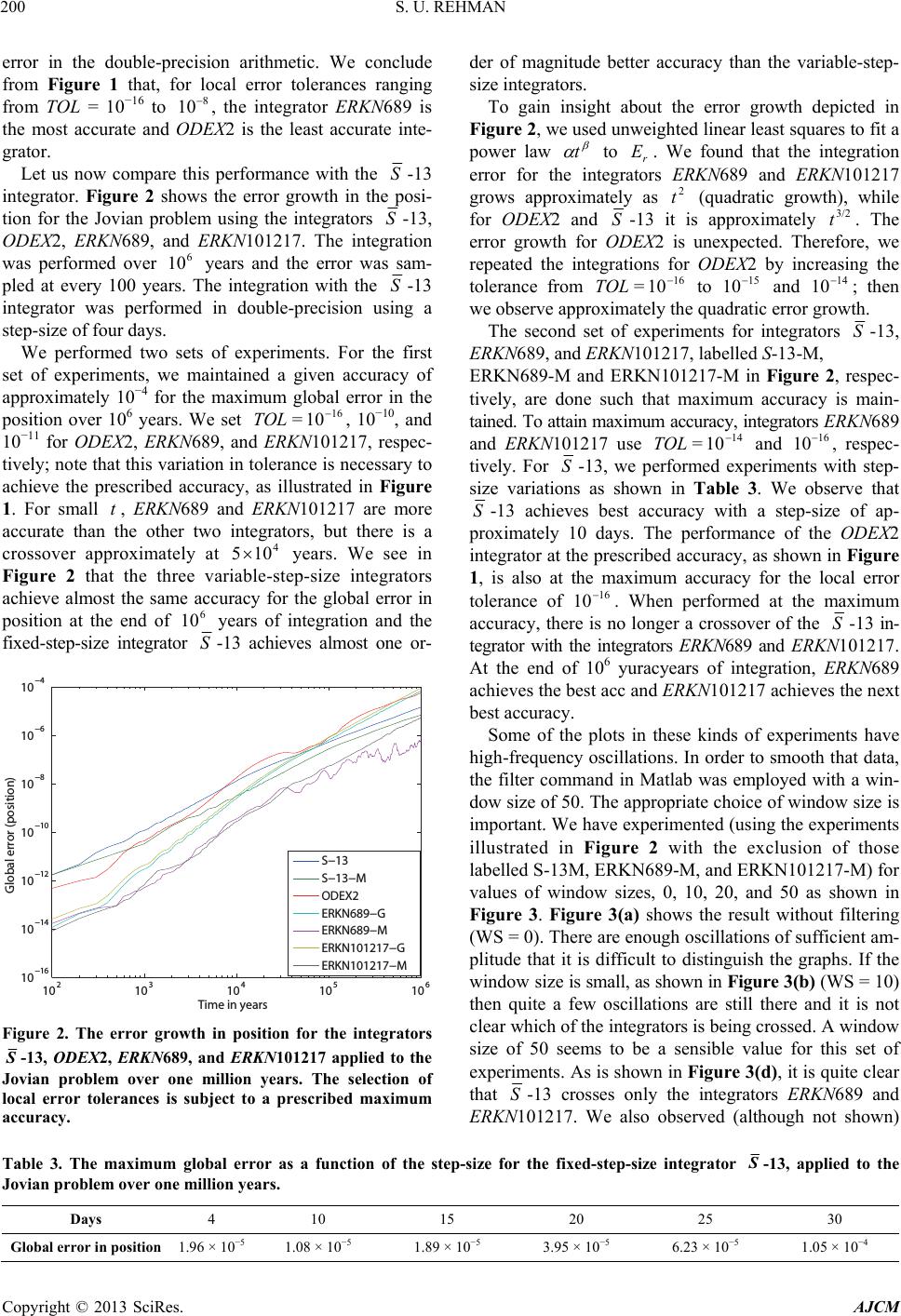

S. U. REHMAN
200
error in the double-precision arithmetic. We conclude
from Figure 1 that, for local error tolerances ranging
from TOL = 10−16 to , the integrator ERKN689 is
the most accurate and ODEX2 is the least accurate inte-
grator.
8
10 
Let us now compare this performance with the S-13
integrator. Figure 2 shows the error growth in the posi-
tion for the Jovian problem using the integrators S-13,
ODEX2, ERKN689, and ERKN101217. The integration
was performed over years and the error was sam-
pled at every 100 years. The integration with the
6
10
S-13
integrator was performed in double-precision using a
step-size of four days.
We performed two sets of experiments. For the first
set of experiments, we maintained a given accuracy of
approximately 10−4 for the maximum global error in the
position over 106 years. We set , 10−10, and
10−11 for ODEX2, ERKN689, and ERKN 101217, respec-
tively; note that this variation in tolerance is necessary to
achieve the prescribed accuracy, as illustrated in Figure
1. For small
16
10=  TOL
t
, ERKN689 and ERKN101217 are more
accurate than the other two integrators, but there is a
crossover approximately at 5 years. We see in
Figure 2 that the three variable-step-size integrators
achieve almost the same accuracy for the global error in
position at the end of years of integration and the
fixed-step-size integrator
4
10
6
10
S-13 achieves almost one or-
10
2
10
3
10
4
10
5
10
6
10
−16
10
−14
10
−12
10
−10
10
−8
10
−6
10
−4
Time in years
Global error (position)
S−13
S−13−M
ODEX2
ERKN689−G
ERKN689−M
ERKN101217−G
ERKN101217−M
Figure 2. The error growth in position for the integrators
S
-13, ODEX2, ERKN689, and ERKN101217 applied to the
Jovian problem over one million years. The selection of
local error tolerances is subject to a prescribed maximum
accuracy.
der of magnitude better accuracy than the variable-step-
size integrators.
To gain insight about the error growth depicted in
Figure 2, we used unweighted linear least squares to fit a
power law to r. We found that the integration
error for the integrators ERKN689 and ERKN101217
grows approximately as (quadratic growth), while
for ODEX2 and

 t E
2
t
S-13 it is approximately . The
error growth for ODEX2 is unexpected. Therefore, we
repeated the integrations for ODEX2 by increasing the
tolerance from to and ; then
we observe approximately the quadratic error growth.
3/2
t
14
1016 10=TOL15 10 
The second set of experiments for integrators S-13,
ERKN689, and ERKN101217, labelled S-13-M,
ERKN689-M and ERKN101217-M in Figure 2, respec-
tively, are done such that maximum accuracy is main-
tained. To attain maximum accuracy, integrators ERKN689
and ERKN101217 use and
14
10=  TOL 16 10

, respec-
tively. For S-13, we performed experiments with step-
size variations as shown in Table 3. We observe that
S-13 achieves best accuracy with a step-size of ap-
proximately 10 days. The performance of the ODEX2
integrator at the prescribed accuracy, as shown in Figure
1, is also at the maximum accuracy for the local error
tolerance of . When performed at the maximum
accuracy, there is no longer a crossover of the
16
10
S-13 in-
tegrator with the integrators ERKN689 and ERKN101217.
At the end of 106 yuracyears of integration, ERKN689
achieves the best acc and ERKN101217 achieves the next
best accuracy.
Some of the plots in these kinds of experiments have
high-frequency oscillations. In order to smooth that data,
the filter command in Matlab was employed with a win-
dow size of 50. The appropriate choice of window size is
important. We have experimented (using the experiments
illustrated in Figure 2 with the exclusion of those
labelled S-13M, ERKN689-M, and ERKN101217-M) for
values of window sizes, 0, 10, 20, and 50 as shown in
Figure 3. Figure 3(a) shows the result without filtering
(WS = 0). There are enough oscillations of sufficient am-
plitude that it is difficult to distinguish the graphs. If the
window size is small, as shown in Figure 3(b) (WS = 10)
then quite a few oscillations are still there and it is not
clear which of the integrators is being crossed. A window
size of 50 seems to be a sensible value for this set of
experiments. As is shown in Figure 3(d), it is quite clear
that S-13 crosses only the integrators ERKN689 and
ERKN101217. We also observed (although not shown)
Table 3. The maximum global error as a function of the step-size for the fixed-step-size integrator
S
-13, applied to the
Jovian problem over one million years.
Days 4 10 15 20 25 30
Global error in position 1.96 × 10−5 1.08 × 10−5 1.89 × 10−5 3.95 × 10−5 6.23 × 10−5 1.05 × 10−4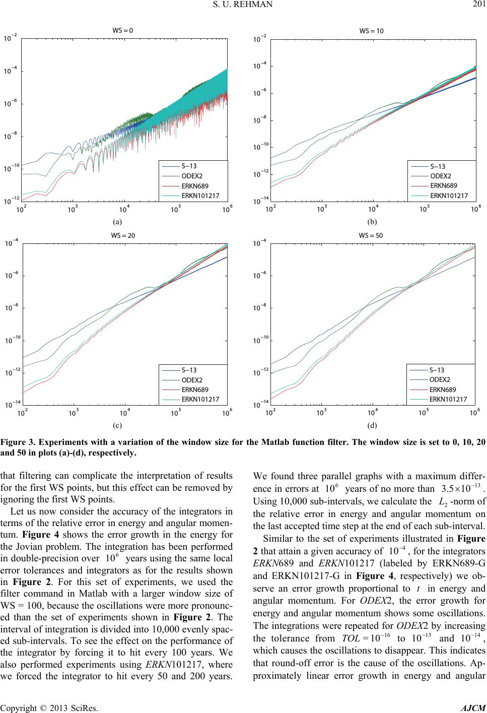

S. U. REHMAN 201
10
2
10
3
10
4
10
5
10
6
10
−12
10
−10
10
−8
10
−6
10
−4
10
−2
WS = 0
S−13
ODEX2
ERKN689
ERKN101217
10
2
10
3
10
4
10
5
10
6
10
−14
10
−12
10
−10
10
−8
10
−6
10
−4
10
−2
WS = 10
S−13
ODEX2
ERKN689
ERKN101217
(a) (b)
10
2
10
3
10
4
10
5
10
6
10
−14
10
−12
10
−10
10
−8
10
−6
10
−4
WS = 20
S−13
ODEX2
ERKN689
ERKN101217
10
2
10
3
10
4
10
5
10
6
10
−14
10
−12
10
−10
10
−8
10
−6
10
−4
WS = 50
S−13
ODEX2
ERKN689
ERKN101217
(c) (d)
Figure 3. Experiments with a variation of the window size for the Matlab function filter. The window size is set to 0, 10, 20
and 50 in plots (a)-(d), respectively.
that filtering can complicate the interpretation of results
for the first WS points, but this effect can be removed by
ignoring the first WS points.
Let us now consider the accuracy of the integrators in
terms of the relative error in energy and angular momen-
tum. Figure 4 shows the error growth in the energy for
the Jovian problem. The integration has been performed
in double-precision over years using the same local
error tolerances and integrators as for the results shown
in Figure 2. For this set of experiments, we used the
filter command in Matlab with a larger window size of
WS = 100, because the oscillations were more pronounc-
ed than the set of experiments shown in Figure 2. The
interval of integration is divided into 10,000 evenly spac-
ed sub-intervals. To see the effect on the performance of
the integrator by forcing it to hit every 100 years. We
also performed experiments using ERKN101217, where
we forced the integrator to hit every 50 and 200 years.
6
10
We found three parallel graphs with a maximum differ-
ence in errors at years of no more than .
Using 10,000 sub-intervals, we calculate the 2-norm of
the relative error in energy and angular momentum on
the last accepted time step at the end of each sub-interval.
6
10 13 103.5 
L
Similar to the set of experiments illustrated in Figure
2 that attain a given accuracy of , for the integrators
ERKN689 and ERKN101217 (labeled by ERKN689-G
and ERKN101217-G in Figure 4, respectively) we ob-
serve an error growth proportional to
4
10
t
in energy and
angular momentum. For ODEX2, the error growth for
energy and angular momentum shows some oscillations.
The integrations were repeated for ODEX2 by increasing
the tolerance from to and ,
which causes the oscillations to disappear. This indicates
that round-off error is the cause of the oscillations. Ap-
proximately linear error growth in energy and angular
16
10=  TOL 15 1014 10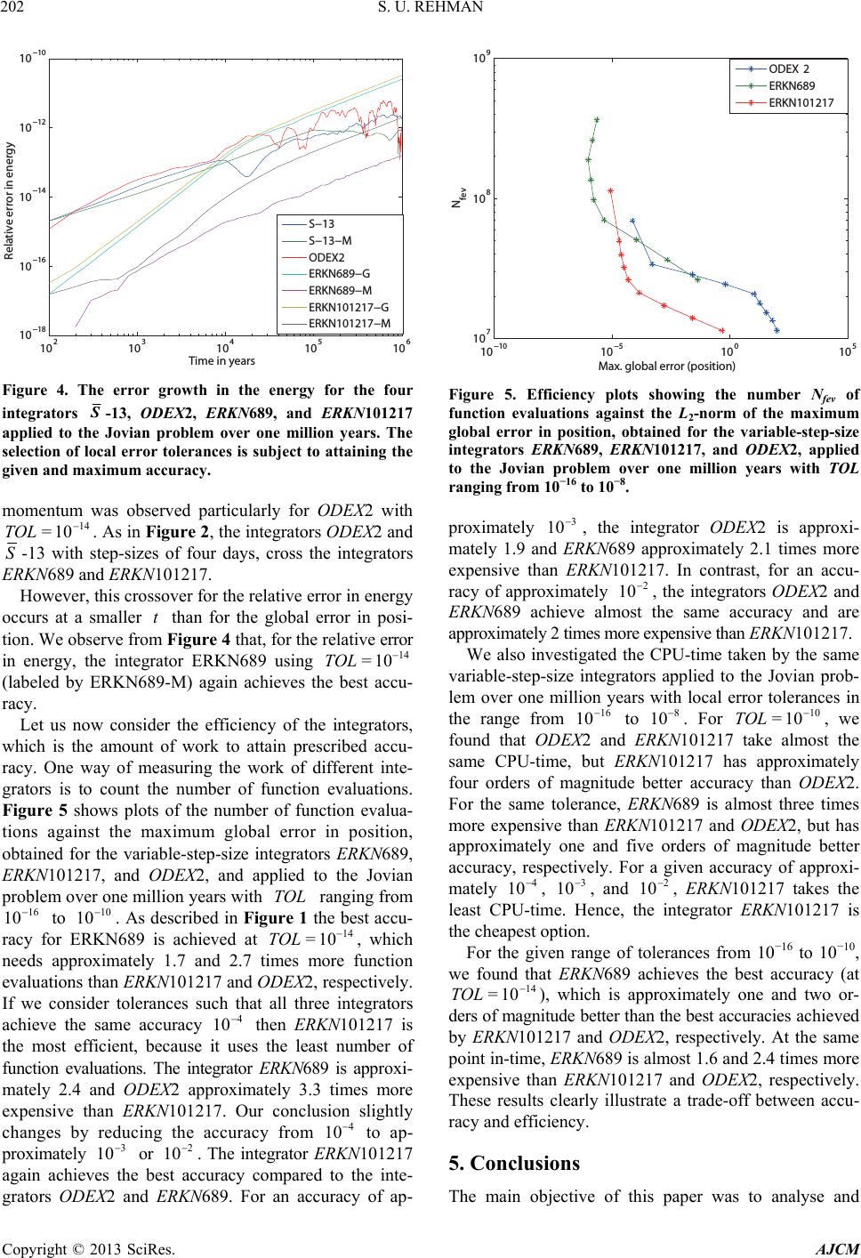

S. U. REHMAN
202
10
2
10
3
10
4
10
5
10
6
10
−18
10
−16
10
−14
10
−12
10
−10
Time in years
Relative error in energy
S−13
S−13−M
ODEX2
ERKN689−G
ERKN689−M
ERKN101217−G
ERKN101217−M
Figure 4. The error growth in the energy for the four
integrators
S
-13, ODEX2, ERKN689, and ERKN101217
applied to the Jovian problem over one million years. The
selection of local error tolerances is subject to attaining the
given and maximum accuracy.
momentum was observed particularly for ODEX2 with
. As in Figure 2, the integrators ODEX2 and
14
10=  TOL
S-13 with step-sizes of four days, cross the integrators
ERKN689 and ERKN101217.
However, this crossover for the relative error in energy
occurs at a smaller
t
than for the global error in posi-
tion. We observe from Figure 4 that, for the relative error
in energy, the integrator ERKN689 using 14 =10TOL

(labeled by ERKN689-M) again achieves the best accu-
racy.
Let us now consider the efficiency of the integrators,
which is the amount of work to attain prescribed accu-
racy. One way of measuring the work of different inte-
grators is to count the number of function evaluations.
Figure 5 shows plots of the number of function evalua-
tions against the maximum global error in position,
obtained for the variable-step-size integrators ERKN689,
ERKN101217, and ODEX2, and applied to the Jovian
problem over one million years with ranging from
to . As described in Figure 1 the best accu-
racy for ERKN689 is achieved at , which
needs approximately 1.7 and 2.7 times more function
evaluations than ERKN101217 and ODEX2, respectively.
If we consider tolerances such that all three integrators
achieve the same accuracy then ERKN101217 is
the most efficient, because it uses the least number of
function evaluations. The integrator ERKN689 is approxi-
mately 2.4 and ODEX2 approximately 3.3 times more
expensive than ERKN101217. Our conclusion slightly
changes by reducing the accuracy from
TOL
TOL
16
10 10 10
14
=10
4
10
4
10

to ap-
proximately or . The integrator ERKN101217
again achieves the best accuracy compared to the inte-
grators ODEX2 and ERKN689. For an accuracy of ap-
3
10 2 10 
10
−10
10
−5
10
0
10
5
10
7
10
8
10
9
Max. global error (position)
N
fev
ODEX 2
ERKN689
ERKN101217
Figure 5. Efficiency plots showing the number Nfev of
function evaluations against the L2-norm of the maximum
global error in position, obtained for the variable-step-size
integrators ERKN689, ERKN101217, and ODEX2, applied
to the Jovian problem over one million years with TOL
ranging from 10−16 to 10−8.
proximately , the integrator ODEX2 is approxi-
mately 1.9 and ERKN689 approximately 2.1 times more
expensive than ERKN101217. In contrast, for an accu-
racy of approximately , the integrators ODEX2 and
ERKN689 achieve almost the same accuracy and are
approximately 2 times more expensive than ERKN101217.
3
10
2
10 
We also investigated the CPU-time taken by the same
variable-step-size integrators applied to the Jovian prob-
lem over one million years with local error tolerances in
the range from to . For , we
found that ODEX2 and ERKN101217 take almost the
same CPU-time, but ERKN101217 has approximately
four orders of magnitude better accuracy than ODEX2.
For the same tolerance, ER KN689 is almost three times
more expensive than ERKN101217 and ODEX2, but has
approximately one and five orders of magnitude better
accuracy, respectively. For a given accuracy of approxi-
mately , , and , ERKN101217 takes the
least CPU-time. Hence, the integrator ERKN101217 is
the cheapest option.
16
10 
3
8
10 
2
10
10
10=  TOL
4
10 10
For the given range of tolerances from 10−16 to 10−10,
we found that ERKN689 achieves the best accuracy (at
), which is approximately one and two or-
ders of magnitude better than the best accuracies achieved
by ERKN101217 and ODEX2, respectively. At the same
point in-time, ERKN689 is almost 1.6 and 2.4 times more
expensive than ERKN101217 and ODEX2, respectively.
These results clearly illustrate a trade-off between accu-
racy and efficiency.
14
10=  TOL
5. Conclusions
The main objective of this paper was to analyse and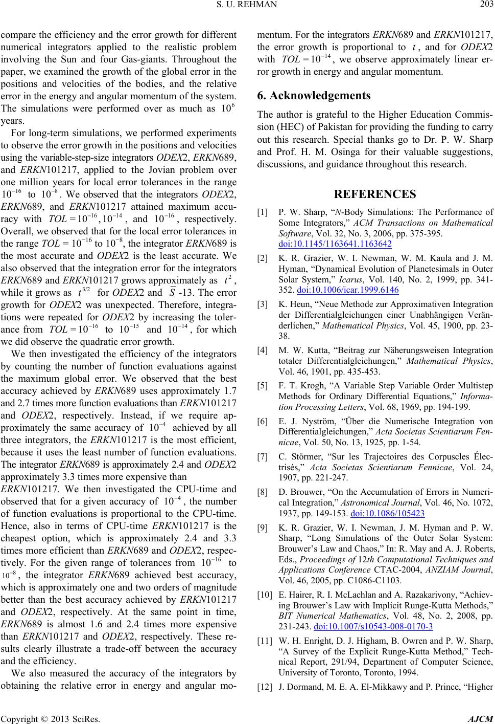

S. U. REHMAN 203
compare the efficiency and the error growth for different
numerical integrators applied to the realistic problem
involving the Sun and four Gas-giants. Throughout the
paper, we examined the growth of the global error in the
positions and velocities of the bodies, and the relative
error in the energy and angular momentum of the system.
The simulations were performed over as much as
years.
6
10
For long-term simulations, we performed experiments
to observe the error growth in the positions and velocities
using the variable-step-size integrators ODEX2, ERKN689,
and ERKN101217, applied to the Jovian problem over
one million years for local error tolerances in the range
to . We observed that the integrators ODEX2,
ERKN689, and ERKN101217 attained maximum accu-
racy with , and , respectively.
Overall, we observed that for the local error tolerances in
the range TOL = 10−16 to 10−8, the integrator ERKN689 is
the most accurate and ODEX2 is the least accurate. We
also observed that the integration error for the integrators
ERKN689 and ERKN101217 grows approximately as ,
while it grows as for ODEX2 and
16
108 10
TO 16 14 =10 ,10L
3/2
t
16
10 
2
t
S-13. The error
growth for ODEX2 was unexpected. Therefore, integra-
tions were repeated for ODEX2 by increasing the toler-
ance from to and , for which
we did observe the quadratic error growth.
16
10= 10TOL 1514 10 
We then investigated the efficiency of the integrators
by counting the number of function evaluations against
the maximum global error. We observed that the best
accuracy achieved by ERKN689 uses approximately 1.7
and 2.7 times more function evaluations than ERKN101217
and ODEX2, respectively. Instead, if we require ap-
proximately the same accuracy of achieved by all
three integrators, the ERKN101217 is the most efficient,
because it uses the least number of function evaluations.
The integrator ERKN689 is approximately 2.4 and ODEX2
approximately 3.3 times more expensive than
ERKN101217. We then investigated the CPU-time and
observed that for a given accuracy of , the number
of function evaluations is proportional to the CPU-time.
Hence, also in terms of CPU-time ERKN101217 is the
cheapest option, which is approximately 2.4 and 3.3
times more efficient than ERKN689 and ODEX2, respec-
tively. For the given range of tolerances from to
, the integrator ERKN689 achieved best accuracy,
which is approximately one and two orders of magnitude
better than the best accuracy achieved by ERKN101217
and ODEX2, respectively. At the same point in time,
ERKN689 is almost 1.6 and 2.4 times more expensive
than ERKN101217 and ODEX2, respectively. These re-
sults clearly illustrate a trade-off between the accuracy
and the efficiency.
4
10
10 4
16
10 
8
10
We also measured the accuracy of the integrators by
obtaining the relative error in energy and angular mo-
mentum. For the integrators ERKN689 and ERKN101217,
the error growth is proportional to
t
, and for ODEX2
with , we observe approximately linear er-
ror growth in energy and angular momentum.
14
10=  TOL
6. Acknowledgements
The author is grateful to the Higher Education Commis-
sion (HEC) of Pakistan for providing the funding to carry
out this research. Special thanks go to Dr. P. W. Sharp
and Prof. H. M. Osinga for their valuable suggestions,
discussions, and guidance throughout this research.
REFERENCES
[1] P. W. Sharp, “N-Body Simulations: The Performance of
Some Integrators,” ACM Transactions on Mathematical
Software, Vol. 32, No. 3, 2006, pp. 375-395.
doi:10.1145/1163641.1163642
[2] K. R. Grazier, W. I. Newman, W. M. Kaula and J. M.
Hyman, “Dynamical Evolution of Planetesimals in Outer
Solar System,” Icarus, Vol. 140, No. 2, 1999, pp. 341-
352. doi:10.1006/icar.1999.6146
[3] K. Heun, “Neue Methode zur Approximativen Integration
der Differentialgleichungen einer Unabhängigen Verän-
derlichen,” Mathematical Physics, Vol. 45, 1900, pp. 23-
38.
[4] M. W. Kutta, “Beitrag zur Näherungsweisen Integration
totaler Differentialgleichungen,” Mathematical Physics,
Vol. 46, 1901, pp. 435-453.
[5] F. T. Krogh, “A Variable Step Variable Order Multistep
Methods for Ordinary Differential Equations,” Informa-
tion Processing Letters, Vol. 68, 1969, pp. 194-199.
[6] E. J. Nyström, “Über die Numerische Integration von
Differentialgleichungen,” Acta Societas Scientiarum Fen-
nicae, Vol. 50, No. 13, 1925, pp. 1-54.
[7] C. Störmer, “Sur les Trajectoires des Corpuscles Élec-
trisés,” Acta Societas Scientiarum Fennicae, Vol. 24,
1907, pp. 221-247.
[8] D. Brouwer, “On the Accumulation of Errors in Numeri-
cal Integration,” Astronomical Journal, Vol. 46, No. 1072,
1937, pp. 149-153. doi:10.1086/105423
[9] K. R. Grazier, W. I. Newman, J. M. Hyman and P. W.
Sharp, “Long Simulations of the Outer Solar System:
Brouwer’s Law and Chaos,” In: R. May and A. J. Roberts,
Eds., Proceedings of 12th Computational Techniques and
Applications Conference CTAC-2004, ANZIAM Journal,
Vol. 46, 2005, pp. C1086-C1103.
[10] E. Hairer, R. I. McLachlan and A. Razakarivony, “Achiev-
ing Brouwer’s Law with Implicit Runge-Kutta Methods,”
BIT Numerical Mathematics, Vol. 48, No. 2, 2008, pp.
231-243. doi:10.1007/s10543-008-0170-3
[11] W. H. Enright, D. J. Higham, B. Owren and P. W. Sharp,
“A Survey of the Explicit Runge-Kutta Method,” Tech-
nical Report, 291/94, Department of Computer Science,
University of Toronto, Toronto, 1994.
[12] J. Dormand, M. E. A. El-Mikkawy and P. Prince, “Higher

S. U. REHMAN
204
Order Embedded Runge-Kutta-Nyström Formulae,” IMA
Journal of Numerical Analysis, Vol. 7, No. 4, 1987, pp.
423-430. doi:10.1093/imanum/7.4.423
[13] L. F. Shampine and M. K. Gordon, “Computer Solution
of Ordinary Differential Equations,” W. H. Freeman, San
Francisco, 1975.
[14] E. Hairer, S. P. Nørsett and G. Wanner, “Solving Ordi-
nary Differential Equations I: Nonstiff Problems,” Sprin-
ger-Verlag, Berlin, 1987.
[15] K. R. Grazier, “The Stability of Planetesimal Niches in
the Outer Solar System: A Numerical Investigation,” PhD
Thesis, University of California, 1997.
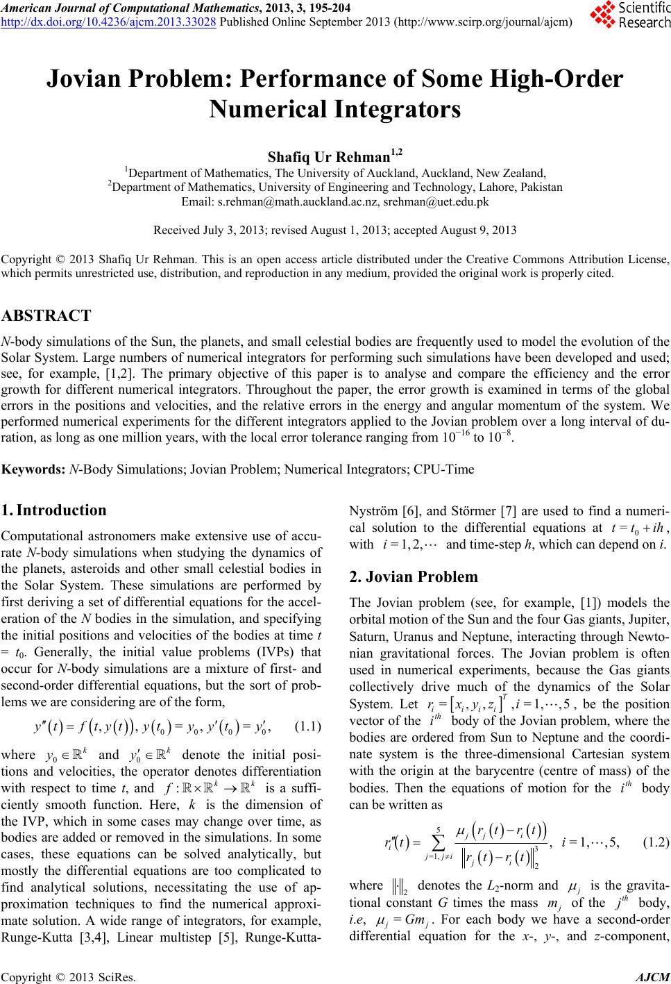