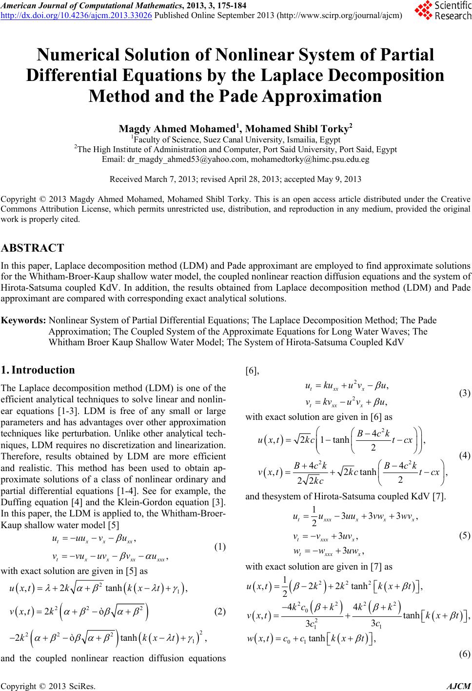
American Journal of Computational Mathematics, 2013, 3, 175-184
http://dx.doi.org/10.4236/ajcm.2013.33026 Published Online September 2013 (http://www.scirp.org/journal/ajcm)
Numerical Solution of Nonlinear System of Partial
Differential Equations by the Laplace Decomposition
Method and the Pade Approximation
Magdy Ahmed Mohamed1, Mohamed Shibl Torky2
1Faculty of Science, Suez Canal University, Ismailia, Egypt
2The High Institute of Administration and Computer, Port Said University, Port Said, Egypt
Received March 7, 2013; revised April 28, 2013; accepted May 9, 2013
Copyright © 2013 Magdy Ahmed Mohamed, Mohamed Shibl Torky. This is an open access article distributed under the Creative
Commons Attribution License, which permits unrestricted use, distribution, and reproduction in any medium, provided the original
work is properly cited.
ABSTRACT
In this paper, Laplace decomposition method (LDM) and Pade approximant are employed to find approximate solutions
for the Whitham-Broer-Kaup shallow water model, the coupled nonlinear reaction diffusion equations and the system of
Hirota-Satsuma coupled KdV. In addition, the results obtained from Laplace decomposition method (LDM) and Pade
approximant are compared with corresponding exact analytical solutions.
Keywords: Nonlinear System of Partial Differential Equations; The Laplace Decomposition Method; The Pade
Approximation; The Coupled System of the Approximate Equations for Long Water Waves; The
Whitham Broer Kaup Shallow Water Model; The System of Hirota-Satsuma Coupled KdV
1. Introduction
The Laplace decomposition method (LDM) is one of the
efficient analytical techniques to solve linear and nonlin-
ear equations [1-3]. LDM is free of any small or large
parameters and has advantages over other approximation
techniques like perturbation. Unlike other analytical tech-
niques, LDM requires no discretization and linearization.
Therefore, results obtained by LDM are more efficient
and realistic. This method has been used to obtain ap-
proximate solutions of a class of nonlinear ordinary and
partial differential equations [1-4]. See for example, the
Duffing equation [4] and the Klein-Gordon equation [3].
In this paper, the LDM is applied to, the Whitham-Broer-
Kaup shallow water model [5]
,
,
txxxx
txxxxx
uuuvu
vvuuvv u
xx


 
  (1)
with exact solution are given in [5] as
 





 
2
1
22 2
2
22 2
1
ò
,2 tanh,
,2
2tanhò,
uxtkkx t
vxt k
kk
 
 
 
 

 
xt
(2)
and the coupled nonlinear reaction diffusion equations
[6],
2
2
,
,
txx x
txx x
uku uvu
vkv uvu



 (3)
with exact solution are given in [6] as


2
22
4
,21tanh ,
2
44
,2tanh
2
22
Bck
uxtkct cx
Bck Bck
vxtkct cx
kc



 







 


,
(4)
and thesystem of Hirota-Satsuma coupled KdV [7].
1333
2
3,
3,
t xxx xxx
t xxxx
t xxxx
uu uuvwwv
vv uv
ww uw

 
 
,
(5)
with exact solution are given in [7] as






 
222
2222
0
2
1 1
01
1
,22tanh ,
2
44
,tanh
3 3
,tanh ,
uxtkkkx t
kckkk
vxtkx t
c c
wxtc ckxt

 



 
  

  

,
(6)
C
opyright © 2013 SciRes. AJCM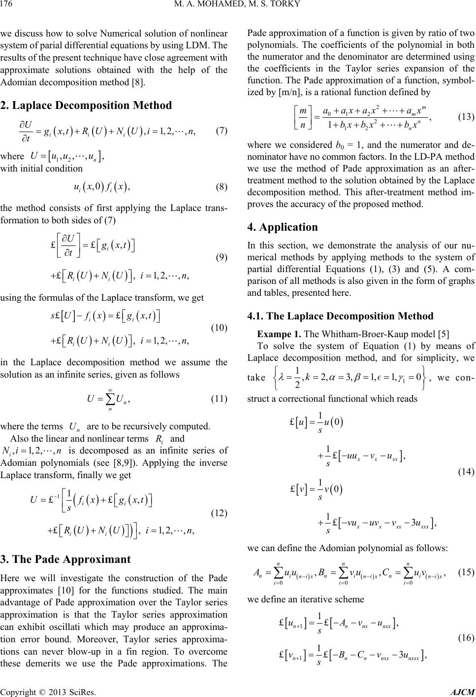

M. A. MOHAMED, M. S. TORKY
176
we discuss how to solve Numerical solution of nonlinear
system of parial differential equations by using LDM. The
results of the present technique have close agreement with
approximate solutions obtained with the help of the
Adomian decomposition method [8].
2. Laplace Decomposition Method
 
,,
iii
U1,2,,,
g
xtR UNUin
t
 
 (7)
where


12
,,, ,
n
Uuu u
with initial condition




,0 ,
ii
ux fx (8)
the method consists of first applying the Laplace trans-
formation to both sides of (7)

 
££,
£,1,
i
ii
Ugxt
t
RU NUin


 
 


  

 2,,,
(9)
using the formulas of the Laplace transform, we get


 
 
££,
£,1,
ii
ii
sU fxgxt
RU NUin
 

 

2,,,
(10)
in the Laplace decomposition method we assume the
solution as an infinite series, given as follows
,
n
n
UU

 (11)
where the terms are to be recursively computed.
n
Also the linear and nonlinear terms i and
is decomposed as an infinite series of
Adomian polynomials (see [8,9]). Applying the inverse
Laplace transform, finally we get
UR
,1,2,,
i
Ni n
 

 

11
££,
£,
ii
ii
Ufxgxt
s
RU NUin


 


 


1,2,,,
(12)
3. The Pade Approximant
Here we will investigate the construction of the Pade
approximates [10] for the functions studied. The main
advantage of Pade approximation over the Taylor series
approximation is that the Taylor series approximation
can exhibit oscillati which may produce an approxima-
tion error bound. Moreover, Taylor series approxima-
tions can never blow-up in a fin region. To overcome
these demerits we use the Pade approximations. The
Pade approximation of a function is given by ratio of two
polynomials. The coefficients of the polynomial in both
the numerator and the denominator are determined using
the coefficients in the Taylor series expansion of the
function. The Pade approximation of a function, symbol-
ized by [m/n], is a rational function defined by
2
01 2
2
12
,
1
m
mn
n
aaxax ax m
nbx bxbx
 


  


 (13)
where we considered b0 = 1, and the numerator and de-
nominator have no common factors. In the LD-PA method
we use the method of Pade approximation as an after-
treatment method to the solution obtained by the Laplace
decomposition method. This after-treatment method im-
proves the accuracy of the proposed method.
4. Application
In this section, we demonstrate the analysis of our nu-
merical methods by applying methods to the system of
partial differential Equations (1), (3) and (5). A com-
parison of all methods is also given in the form of graphs
and tables, presented here.
4.1. The Laplace Decomposition Method
Exampe 1. The Whitham-Broer-Kaup model [5]
To solve the system of Equation (1) by means of
Laplace decomposition method, and for simplicity, we
take 1
1,2,3,1,1, 0
2k







, we con-
struct a correctional functional which reads






1
£0
1£,
1
£0
1£3
xxxx
xxxxxxx
uu
s
uuvu
s
vv
s
vu uv vu
s



 ,
,

(14)
we can define the Adomian polynomial as follows:
  
000
,,
nnn
ni ni ni
nix nix nix
iii
AuuBvuCuv




(15)
we define an iterative scheme
 
 
1
1
1
££ ,
1
££ 3
nn nxnxx
nnn nxxnxxx
uAvu
s
vBCvu
s



 ,
(16)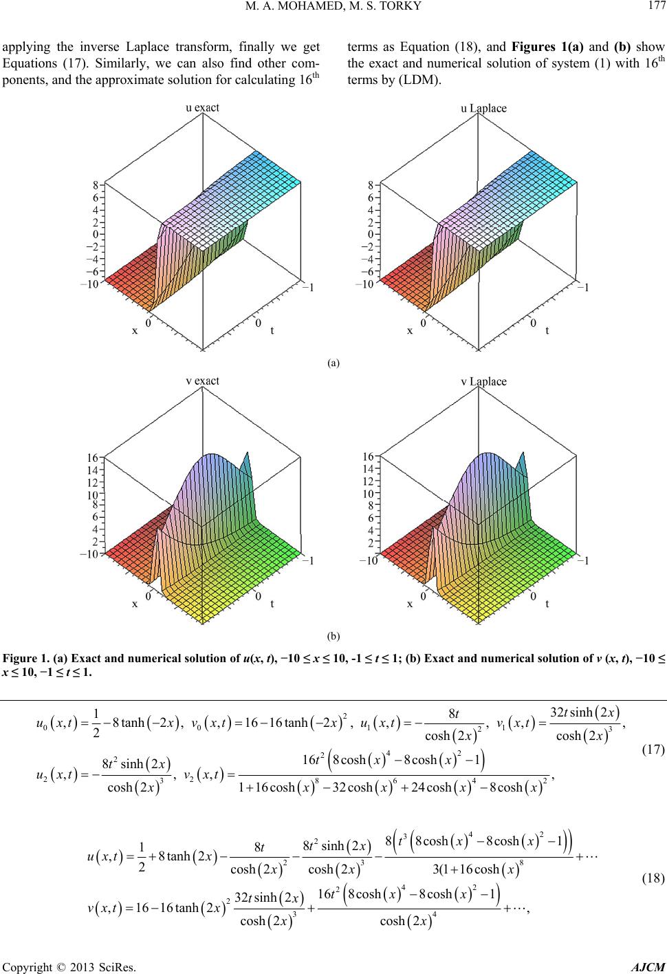

M. A. MOHAMED, M. S. TORKY
177
terms as Equation (18), and Figures 1(a) and (b) show
the exact and numerical solution of system (1) with 16th
terms by (LDM).
applying the inverse Laplace transform, finally we get
Equations (17). Similarly, we can also find other com-
ponents, and the approximate solution for calculating 16th
(a)
(b)
Figure 1. (a) Exact and numerical solution of u(x, t), −10 ≤ x ≤ 10, -1 ≤ t ≤ 1; (b) Exact and numerical solution of v (x, t), −10 ≤
x ≤ 10, −1 ≤ t ≤ 1.
    

 
   

 
2
00 11
23
42
2
2
22
38642
32 sinh2
18
,8tanh2,,1616tanh2,,,,
2cosh 2cosh 2
16 8cosh8cosh1
8sinh2
,,, ,
cosh2116 cosh32 cosh24 cosh8 cosh
tx
t
uxtx vxtxuxtvxt
xx
tx x
tx
uxt vxt
xxxxx
 

  
,
(17)
  


 





 

 


42
3
2
23 8
42
2
2
34
88cosh8cosh 1
8sinh2
18
,8tanh2
2cosh2cosh23(116 cosh
16 8cosh8cosh1
32 sinh2
,1616tanh2 ,
cosh 2cosh 2
tx x
tx
t
uxtx xx x
tx x
tx
vxtx xx

 


 


(18)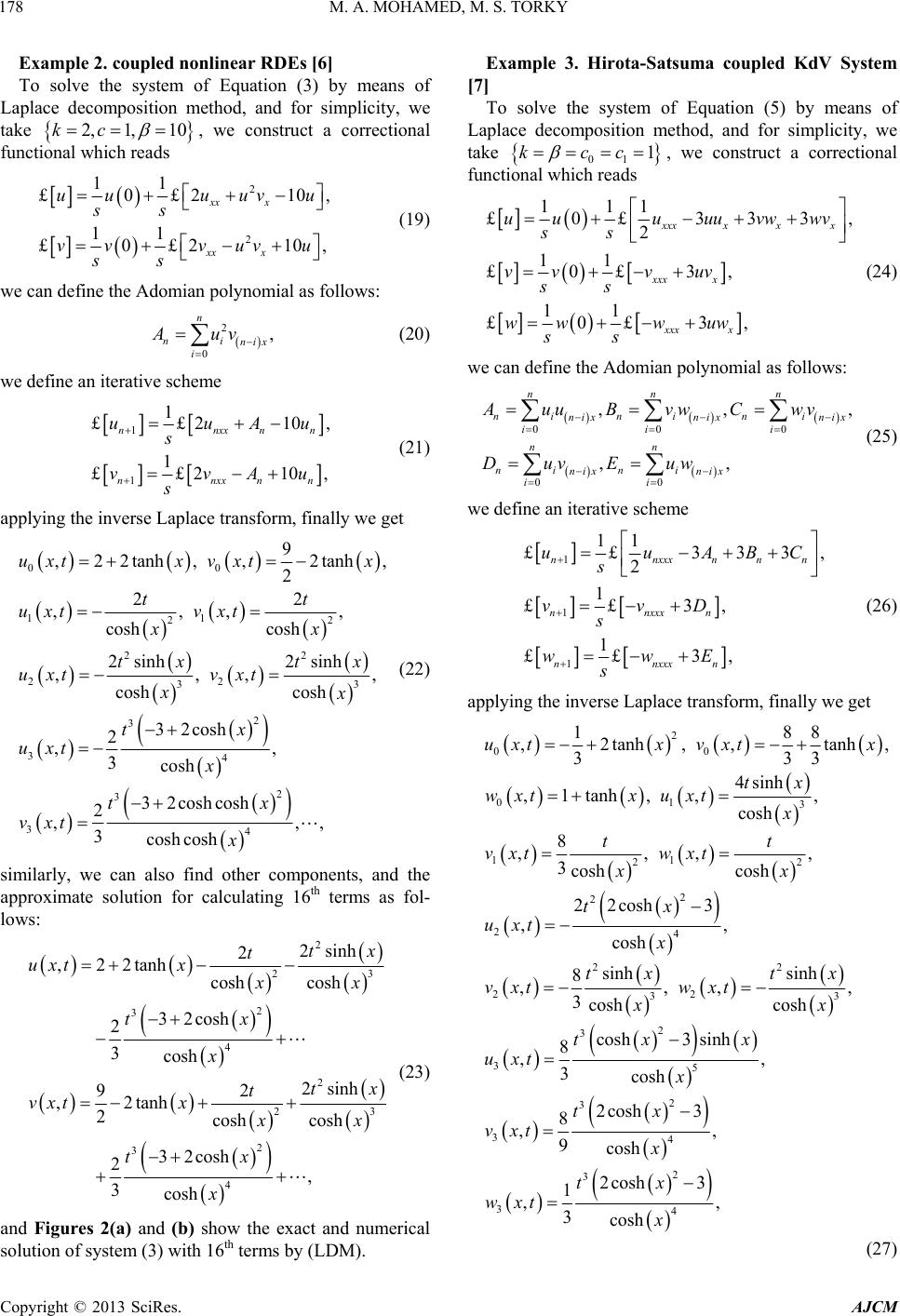

M. A. MOHAMED, M. S. TORKY
178
Example 2. coupled nonlinear RDEs [6]
To solve the system of Equation (3) by means of
Laplace decomposition method, and for simplicity, we
take , we construct a correctional
functional which reads

2, 1,10kc  



 
2
2
11
£02 10
11
£02 10
£
,£
xx x
xx x
uu uuvu
ss
vv vuvu
ss

 


 

,
(19)
we can define the Adomian polynomial as follows:

2
0
,
n
ni
nix
i
Auv


 (20)
we define an iterative scheme
 
 
1
1
1
££2 10
1
££2 10
nnxxn
nnxxn
uuA
s
vvA
s




,
,
n
n
u
u
(21)
applying the inverse Laplace transform, finally we get

   
 
   
 


 


00
11
22
22
22
33
2
3
34
2
3
34
9
,22tanh, ,2tanh
2
22
,,,
cosh cosh
2sinh2sinh
,,,
cosh cosh
32cosh
2
,,
3cosh
32cosh cosh
2
,,
3cosh cosh
uxtx vxtx
tt
uxt vxt
xx
tx tx
uxt vxt
x
tx
uxt x
tx
vxt x
 
 
 




,
,
,
,
x
(22)
similarly, we can also find other components, and the
approximate solution for calculating 16th terms as fol-
lows:
 






  





2
23
2
3
4
2
23
2
3
4
2sinh
2
,22tanh
cosh cosh
32cosh
2
3cosh
2sinh
92
,2tanh
2cosh cosh
32cosh
2,
3cosh
tx
t
uxtxxx
tx
x
tx
t
vxt x
x
x
tx
x
 


 




(23)
and Figures 2(a) and (b) show the exact and numerical
solution of system (3) with 16th terms by (LDM).
Example 3. Hirota-Satsuma coupled KdV System
[7]
To solve the system of Equation (5) by means of
Laplace decomposition method, and for simplicity, we
take


01
1kcc 

, we construct a correctional
functional which reads
 






111
£0 33£
£
£
3,
2
11
£0 3,
11
£0 3,
xxx xxx
xxx x
xxx x
uuu uuvwwv
ss
vvvuv
ss
wwwuw
ss


 






(24)
we can define the Adomian polynomial as follows:
  
 
00 0
00
,,
,,
nn n
ninin i
nix nix nix
ii i
nn
ni ni
nix nix
ii
AuuBvwCwv
DuvE uw

 






,

(25)
we define an iterative scheme

 
 
1
1
1
11
££333
2
1
££3,
1
££3,
nnxxx n nn
nnxxxn
nnxxxn
uuAB
s
vvD
s
wwE
s



,C









(26)
applying the inverse Laplace transform, finally we get
  


  
 


 
   
 



2
00
01
3
11
22
2
2
24
22
22
33
2
3
35
18
,2 tanh,,tanh,
33
4sinh
,1tanh, ,,
cosh
8
,,,,
3cosh cosh
22cosh 3
,,
cosh
sinh sinh
8
,,,
3cosh cosh
cosh3sinh
8
,,
3cos h
uxtx vxtx
tx
wxtx uxtx
tt
vxt wxt
xx
tx
uxt x
tx tx
vxt wxt
xx
tx x
uxt x
  
 



 



8
3
,



 


2
3
34
2
3
34
2cosh3
8
,,
9cosh
2cosh 3
1
,,
3cosh
tx
vxt x
tx
wxt x




(27)

M. A. MOHAMED, M. S. TORKY 179
(a)
(b)
Figure 2. (a) Exact and numerical solution of u(x, t), −10 ≤ x ≤ 10, −1 ≤ t ≤ 1; (b) Exact and numerical solution of v(x, t), −10 ≤
x ≤ 10, −1 ≤ t ≤ 1.
similarly, we can also find other components, and the ap-
proximate solution for calculating 16th terms as follows:
  








  








 




2
3
22
23
45
2
3
22
23
45
2
23
2
3
4sinh
1
,2tanh
3cosh
22cosh 3cosh3sinh
8
3
cosh cosh
4sinh
1
,2tanh
3cosh
22cosh 3cosh3sinh
8
3
cosh cosh
sinh
,1tanh
cosh cosh
2cosh 3
1
3co
tx
uxtx x
tx txx
xx
tx
vxtx x
tx txx
xx
tx
t
wxtx xx
tx
 


 


 





and Figures 3(a)-(c) show the exact and numerical so-
lution of system (5) with 16th terms by (LDM).
4.2. The Pade Approximation


4,
sh x
(28)
In this section we use Maple to calculate the [3/2] the Pade
approximant of the infinite series solution (18), (23), and
(28) which gives the rational fraction approximation to the
solution, and Figures 4(a)-(c) show the results obtained
by the Pade approximant (LD-PA) solution of systems (1),
(3) and (5), and Figures 5(a)-(c) show comparison be-
tween the exact solution, LDM solution and the Pade
approximant (LD-PA) solution of systems (1), (3) and (5)
at, x = 5, −1 ≤ t ≤ 1. Tables 1-3 show the absolute error
between the exact solution and the results obtained from
the, LDM solution and the Pade approximant (LD-PA)
solution of systems (1)-(3).
5. Conclusion
The Laplace decomposition method is a powerful tool

M. A. MOHAMED, M. S. TORKY
180
(a)
(b)
(c)
Figure 3. (a) Exact and numerical solution of u(x, t), −10 ≤ x ≤ 10, −1 ≤ t ≤ 1; (b) Exact and numerical solution of v(x, t), −10 ≤
x ≤ 10, −1 ≤ t ≤ 1; (c) Exact and numerical solution of w(x, t), −10 ≤ x ≤ 10, −1 ≤ t ≤ 1.

M. A. MOHAMED, M. S. TORKY 181
(a)
(b)
(c)
Figure 4. (a) The Pade approximant (LD-PA) solution of u(x, t) and v(x, t) of example 1, −10 ≤ x ≤ 10, −1 ≤ t ≤ 1; (b) The Pade
approximant (LD-PA) solution of u(x, t) and v(x, t) of example 2, −10 ≤ x ≤ 10, −1 ≤ t ≤ 1; (c) The Pade approximant (LD-PA)
solution of u(x, t) and v(x, t) and w(x, t) of example 3, −10 ≤ x ≤ 10, −1 ≤ t ≤ 1.

M. A. MOHAMED, M. S. TORKY
182
(a)
(b)
(c)
Figure 5. (a) The exact, (LDM)and the Pade approximant (LD-PA) solution of u(x, t) and v(x, t) of example 1, x = 5, −1 ≤ t ≤ 1;
(b) The exact, (LDM)and the Pade approximant (LD-PA) solution of u(x, t) and v(x, t) of example 2, x = 5, −1 ≤ t ≤ 1; (c) The
exact, (LDM)and the Pade approximant (LD-PA) solution of u(x, t), v(x, t) and w(x, t) of example 3, x = 5, −1 ≤ t ≤ 1.
which is capable of handling nonlinear system of partial
differential equations. In this paper the (LDM) and Pade
approximant has been successfully applied to find ap-
proximate solutions for,the Whitham-Broer-Kaup shal-
low water model, the coupled nonlinear reaction diffu-
sion equations and thesystem of Hirota-Satsuma coupled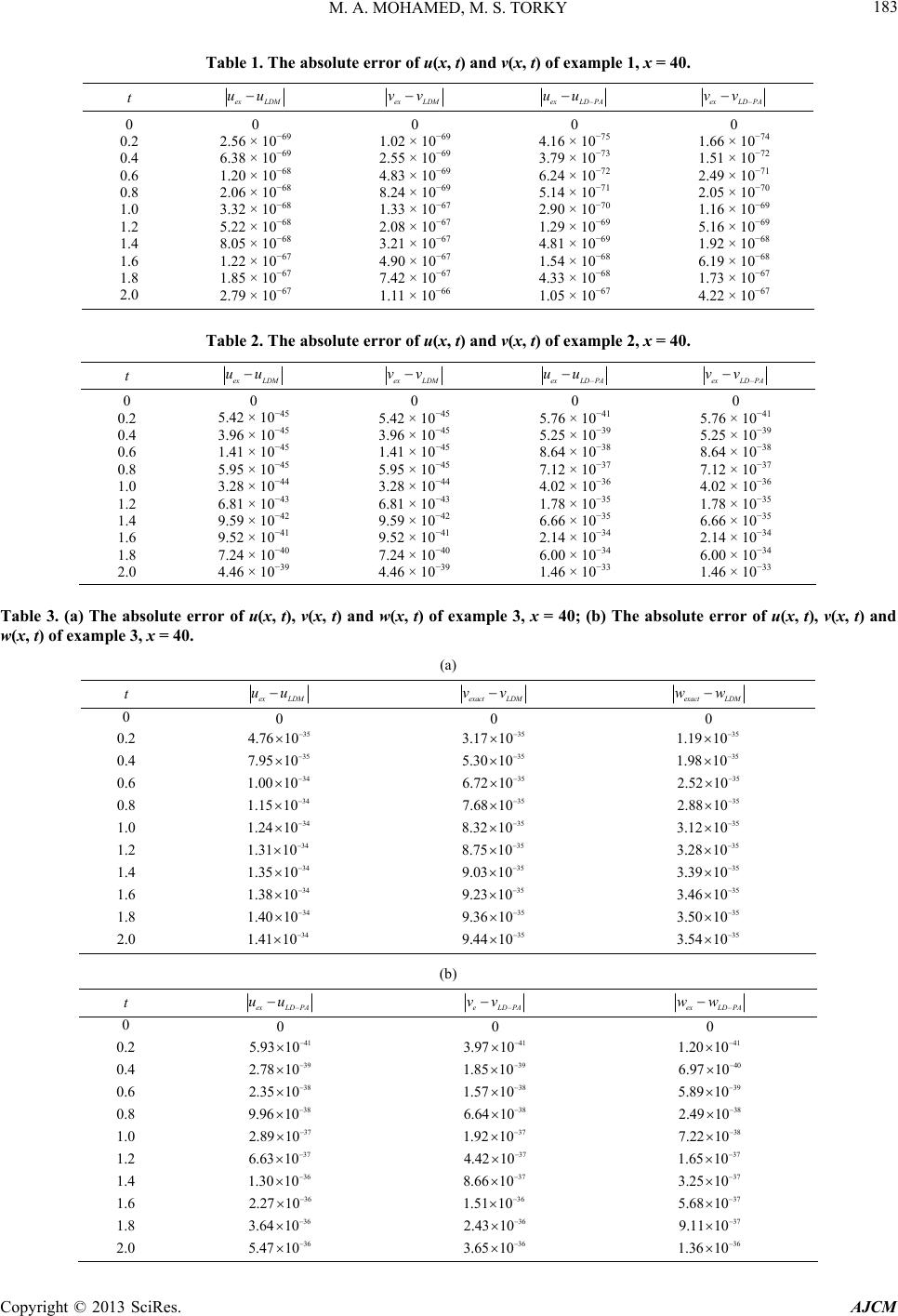

M. A. MOHAMED, M. S. TORKY 183
Table 1. The absolute error of u(x, t) and v(x, t) of example 1, x = 40.
t exLDM
uu exLDM vv –exLD PA uu –exLD PA vv
0
0.2
0.4
0.6
0.8
1.0
1.2
1.4
1.6
1.8
2.0
0
2.56 × 10−69
6.38 × 10−69
1.20 × 10−68
2.06 × 10−68
3.32 × 10−68
5.22 × 10−68
8.05 × 10−68
1.22 × 10−67
1.85 × 10−67
2.79 × 10−67
0
1.02 × 10−69
2.55 × 10−69
4.83 × 10−69
8.24 × 10−69
1.33 × 10−67
2.08 × 10−67
3.21 × 10−67
4.90 × 10−67
7.42 × 10−67
1.11 × 10−66
0
4.16 × 10−75
3.79 × 10−73
6.24 × 10−72
5.14 × 10−71
2.90 × 10−70
1.29 × 10−69
4.81 × 10−69
1.54 × 10−68
4.33 × 10−68
1.05 × 10−67
0
1.66 × 10−74
1.51 × 10−72
2.49 × 10−71
2.05 × 10−70
1.16 × 10−69
5.16 × 10−69
1.92 × 10−68
6.19 × 10−68
1.73 × 10−67
4.22 × 10−67
Table 2. The absolute error of u(x, t) and v(x, t) of example 2, x = 40.
t ex LDM
uu ex LDM vv –exLD PA uu –exLD PA vv
0
0.2
0.4
0.6
0.8
1.0
1.2
1.4
1.6
1.8
2.0
0
5.42 × 10−45
3.96 × 10−45
1.41 × 10−45
5.95 × 10−45
3.28 × 10−44
6.81 × 10−43
9.59 × 10−42
9.52 × 10−41
7.24 × 10−40
4.46 × 10−39
0
5.42 × 10−45
3.96 × 10−45
1.41 × 10−45
5.95 × 10−45
3.28 × 10−44
6.81 × 10−43
9.59 × 10−42
9.52 × 10−41
7.24 × 10−40
4.46 × 10−39
0
5.76 × 10−41
5.25 × 10−39
8.64 × 10−38
7.12 × 10−37
4.02 × 10−36
1.78 × 10−35
6.66 × 10−35
2.14 × 10−34
6.00 × 10−34
1.46 × 10−33
0
5.76 × 10−41
5.25 × 10−39
8.64 × 10−38
7.12 × 10−37
4.02 × 10−36
1.78 × 10−35
6.66 × 10−35
2.14 × 10−34
6.00 × 10−34
1.46 × 10−33
Table 3. (a) The absolute error of u(x, t), v(x, t) and w(x, t) of example 3, x = 40; (b) The absolute error of u(x, t), v(x, t) and
w(x, t) of example 3, x = 40.
(a)
t exLDM
uu exactLDM vv exactLDM ww
0
0.2
0.4
0.6
0.8
1.0
1.2
1.4
1.6
1.8
2.0
0
35
4.76 10 
35
7.95 10 
34
1.00 10 
34
1.15 10 
34
1.24 10 
34
1.31 10 
 34
1.35 10
34
1.38 10
34
1.40 10
34
1.41 10
0
35
3.17 10 
35
5.30 10 
35
6.72 10 
35
7.68 10 
35
8.32 10 
35
8.75 10 
 35
9.03 10
35
9.23 10
35
9.36 10
35
9.44 10
0
35
1.19 10 
35
1.98 10 
35
2.52 10 
35
2.88 10 
35
3.12 10 
35
3.28 10 
 35
3.39 10
35
3.46 10
35
3.50 10
35
3.54 10
(b)
t –exLD PA
uu –eLDPA vv –exLD PA ww
0
0.2
0.4
0.6
0.8
1.0
1.2
1.4
1.6
1.8
2.0
0
41
5.93 10 
39
2.78 10 
38
2.35 10 
38
9.96 10 
37
2.89 10 
37
6.63 10 
 36
1.30 10
36
2.27 10
36
3.64 10
36
5.47 10
0
41
3.97 10 
39
1.85 10 
38
1.57 10 
38
6.64 10 
37
1.92 10 
37
4.42 10 
 37
8.66 10
36
1.51 10
36
2.43 10
36
3.65 10
0
41
1.20 10 
40
6.97 10 
39
5.89 10 
38
2.49 10 
38
7.22 10 
37
1.65 10 
 37
3.25 10
37
5.68 10
37
9.11 10
36
1.36 10

M. A. MOHAMED, M. S. TORKY
184
KdV. It was noted that the scheme found the solutions
without any discretization or restrictive assumption, and
it was free from round-off errors and therefore reduced
the numerical computations to a great extent.
REFERENCES
[1] S. A. Khuri, “A Laplace Decomposition Algorithm Ap-
plied to Class of Nonlinear Differential Equations,” Jour-
nal of Applied Mathematics, Vol. 1, No. 4, 2001, pp. 141-
155.
[2] H. Hosseinzadeh, H. Jafari and M. Roohani, “Application
of Laplace Decomposition Method for Solving Klein-
Gordon Equation,” World Applied Sciences Journal, Vol.
8, No. 7, 2010, pp. 809-813.
[3] M. Khan, M. Hussain, H. Jafari and Y. Khan, “Applica-
tion of Laplace Decomposition Method to Solve Nonlin-
ear Coupled Partial Differential Equations,” World Ap-
plied Sciences Journal, Vol. 9, No. 1, 2010, pp. 13-19.
[4] E. Yusufoglu (Aghadjanov), “Numerical Solution of Duff-
ing Equation by the Laplace Decomposition Algorithm,”
Applied Mathematics and Computation, Vol. 177, No. 2,
2006, pp. 572-580. doi:10.1016/j.amc.2005.07.072
[5] T. Xu, J. Li and H.-Q. Zhang, “New Extension of the
Tanh-Function Method and Application to the Whitham-
Broer-Kaup Shallow Water Model with Symbolic Com-
putation,” Physics Letters A , Vol. 369, No. 5-6, 2007, pp.
458-463. doi:10.1016/j.physleta.2007.05.047
[6] A. A. Solimana and M. A. Abdoub, “Numerical Solutions
of Nonlinear Evolution Equations Using Variational It-
eration Method,” Journal of Computational and Applied
Mathematics, Vol. 207, No. 1, 2007, pp. 111-120.
doi:10.1016/j.cam.2006.07.016
[7] E. Fan, “Soliton Solutions for a Generalized Hirota-Sa-
tsuma Coupled KdV Equation and a Coupled MKdV
Equation,” Physics Letters A, Vol. 2852, No. 1-2, 2001,
pp. 18-22. doi:10.1016/S0375-9601(01)00161-X
[8] H. Jafari and V. Daftardar-Gejji, “Solving Linear and
Nonlinear Fractional Diffution and Wave Equations by
Adomian Decomposition,” Applied Mathematics and Com-
putation, Vol. 180, No. 2, 2006, pp. 488-497.
doi:10.1016/j.amc.2005.12.031
[9] F. Abdelwahid, “A Mathematical Model of Adomian
Polynomials,” Applied Mathematics and Computation,
Vol. 141, No. 2-3, 2003, pp. 447-453.
doi:10.1016/S0096-3003(02)00266-7
[10] T. A. Abassya, M. A. El-Tawil and H. El-Zoheiry, “Exact
Solutions of Some Nonlinear Partial Differential Equa-
tions Using the Variational Iteration Method Linked with
Laplace Transforms and the Pade Technique,” Computers
and Mathematics with Applications, Vol. 54, No. 7-8,
2007, pp. 940-954. doi:10.1016/j.camwa.2006.12.067