Journal of Environmental Protection, 2013, 4, 28-39
http://dx.doi.org/10.4236/jep.2013.48A1005 Published Online August 2013 (http://www.scirp.org/journal/jep)
Artificial Neural Network Modeling of Healthy Risk Level
Induced by Aircraft Pollutant Impacts around Soekarno
Hatta International Airport
Salah Khardi1, Jermanto Setia Kurniawan2, Irwan Katili2, Setyo Moersidik2
1Transports and Environment Laboratory, French Institute of Science and Technology for Transport, Development and Networks
(IFSTTAR), Bron, France; 2Department of Civil Engineering, Faculty of Engineering, University of Indonesia, Kampus Baru UI,
Depok, Indonesia.
Received May 30th, 2013; revised July 2nd, 2013; accepted August 1st, 2013
Copyright © 2013 Salah Khardi et al. This is an open access article distributed under the Creative Commons Attribution License,
which permits unrestricted use, distribution, and reproduction in any medium, provided the original work is properly cited.
ABSTRACT
Aircraft pollutant emissions are an important part of sources of pollution that directly or indirectly affect human health
and ecosystems. This research suggests an Artificial Neural Network model to determine the healthy risk level around
Soekarno Hatta International Airport-Cengkareng Indonesia. This ANN modeling is a flexible method, which enables to
recognize highly complex non-linear correlations. The network was trained with real measurement data and updated
with new measurements, enhancing its quality and making it the ideal method for this research. Measurements of air-
craft pollutant emissions are carried out with the aim to be used as input data and to validate the developed model. The
obtained results concerned the improved ANN architecture model based on pollutant emissions as input variables. ANN
model processes variables—hidden layers—and gives an output variable corresponding to a healthy risk level. This
model is characterized by a 4-10-1 scheme. Based on ANN criteria, the best validation performance is achieved at ep-
och 28 from 34 epochs with the Mean Squared Error (MSE) of 9 × 10−3. The correlation between targets and outputs is
confirmed. It validated a close relationship between targets and outputs. The network output errors value approaches
zero. Further research is needed with the aim to enlarge the scheme of the ANN model by increasing its input variables.
This is one of the major key defining environmental capacities of an airport that should be applied by Indonesian airport
authorities. These would institute policies to manage or reduce pollutant emissions considering population and income
growth to be socially positive.
Keywords: Aircraft; Pollutant Emissions; Artificial Neural Network; Healthy Risk Level
1. Introduction
The continuing growth in air traffic and increasing public
awareness have made environmental considerations one
of the most critical aspects of commercial aviation. It is
generally accepted that significant improvements to the
environmental acceptability of aircraft will be needed if
the long-term growth of air transport is to be sustained.
This is an open issue. The release of exhaust gasses in
the atmosphere is the second major environmental issue
associated with commercial airliners. The expected dou-
bling of the fleet in the next twenty years will certainly
exacerbate the issue: the contribution of aviation is ex-
pected to increase by factor of 1.6 to 10, depending on
the fuel use scenario. Being conscious of this problem,
engine manufacturers have developed low-emission
combustors, and made them available as options. These
combustors have been adopted by airlines operating in
European airports with strict emissions controls, in Swe-
den and Switzerland, for example. Significant progress has
been made with some individual pollutants rather than
with others. Aircraft emissions have also declined over
time when consider the emissions from transporting one
passenger one mile. Current emissions regulations have
focused on local air quality in the vicinity of airports and
the research will also focus on the local impact of Avia-
tion [1,2]. Emissions released during cruise in the upper
atmosphere are recognized as an important issue with
potentially severe long-term environmental consequences,
and ICAO is actively seeking support for regulating them

Artificial Neural Network Modeling of Healthy Risk Level Induced by Aircraft
Pollutant Impacts around Soekarno Hatta International Airport
29
as well. Operations of aircraft are usually divided into two
main parts [3]: The Landing-Take-off (LTO) cycle which
includes all activities near the airport that take place below
the altitude of 3000 feet (914 m). This therefore includes
taxi-in and out, take-off, climb-out and approach-landing.
Cruise is defined as an activity that takes place at alti-
tude above 3000 feet (914 m). No upper limit altitude is
given. Cruise includes climb from the end of climb-out in
the LTO cycle to the cruise altitude, cruise, and descent
from cruise altitudes to the start of LTO operations of
landing. Emissions from aircraft originate from fuel
burned in aircraft engines [3]. Aircraft jet engines pro-
duce carbon dioxide (CO2), water vapor (H2O), Nitrogen
Oxides (NOx), Carbon Monoxide (CO), Oxides of sulfur
(SOx), unburned or partially combusted hydrocarbons
(also known as volatile organic compounds (VOC), par-
ticulates and other trace compounds [4]. A small subset
of the VOCs and particulates are considered hazardous
air pollutants (HAPs).
Aircraft engine emissions are roughly composed of
about 70% CO2, a little less than 30% H2O, and less than
1% each of NOx, CO, SOx, VOC, particulates, and other
trace components including HAPs. Aircraft emissions,
depending on whether they occur near the ground or at
altitude, are primarily considered local air quality pol-
lutants or greenhouse gases [4,5]. Water in the aircraft
exhaust at altitude may have a greenhouse effect, and
occasionally this water produces contrails, which also
may have a greenhouse effect. About 10% of aircraft
emissions of all types, except hydrocarbons and CO [6],
are produced during airport ground level operations and
during landing and takeoff. The bulk of aircraft emis-
sions (90%) occur at higher altitudes [4,7]. For hydro-
carbons and CO, the split is closer to 30% ground level
emissions and 70% at higher altitudes. Aircraft is not the
only source of aviation emissions. Airport access and
ground support vehicles produce similar emissions. Such
vehicles include traffic to and from the airport, ground
equipment that services aircraft, and shuttle buses and
vans serving passengers.
Other emissions sources at the airport include auxiliary
power units providing electricity and air conditioning to
aircraft parked at airport terminal gates, stationary airport
power sources, and construction equipment operating on
the airport [4,8]. Emission from Combustion Processes
CO2—Carbon dioxide is the product of complete com-
bustion of hydrocarbon fuels like gasoline, jet fuel, and
diesel. Carbon in fuel combines with oxygen in the air to
produce CO2. H2O-Water vapor is the other product of
complete combustion as hydrogen in the fuel combines
with oxygen in the air to produce H2O. NOx—Nitrogen
oxides are produced when air passes through high tem-
perature/high pressure combustion and nitrogen and
oxygen present in the air combine to form NOx [4,5,8,9].
HC-Hydrocarbons are emitted due to incomplete fuel
combustion [6]. They are also referred to as volatile or-
ganic compounds (VOCs). Many VOCs are also hazard-
ous air pollutants. CO-Carbon monoxide is formed due to
the incomplete combustion of the carbon in the fuel.
SOx-Sulfur oxides are produced when small quantities of
sulfur, present in essentially all hydrocarbon fuels, com-
bine with oxygen from the air during combustion [4,8].
Particulates—small particles that form as a result of
incomplete combustion, and are small enough to be in-
haled, are referred to as particulates. Particulates can be
solid or liquid. Ozone—O3 is not emitted directly into the
air but is formed by the reaction of VOCs and NOx in the
presence of heat and sunlight [5,9]. Ozone forms readily
in the atmosphere and is the primary constituent of smog.
For this reason it is an important consideration in the
environmental impact of aviation [4,8]. Compared to
other sources, aviation emissions are a relatively small
contributor to air quality concerns both with regard to
local air quality and greenhouse gas emissions. While
small, however, aviation emissions cannot be ignored
[4,8]. Emissions will be dependent on the fuel type, air-
craft type, engine type, engine load and flying altitude.
Two types fuel are used. Gasoline is used in small piston
engines aircraft only. Most aircraft run on kerosene and
the bulk of fuel used for aviation is kerosene. In general,
there exist two types of engines: reciprocating piston
engines and gas turbines [1-3,10-14].
Most emissions originate from the first category which
covers the scheduled flights of ordinary aircraft. The
ICAO is a United Nations intergovernmental body re-
sponsible for worldwide planning, implementation, and
coordination of civil aviation. ICAO sets emission stan-
dards for jet engines. These are the basis of FAA’s air-
craft engine performance certification standards, estab-
lished through EPA regulations. Currently ICAO has
covered three approaches to quantifying aircraft engine
emissions: two in detail and one in overview: Simple
Approach, Advanced Approach and Sophisticated Ap-
proach [1,2,11-13,15,16]:
 Simple Approach is the least complicated approach,
requires the minimum amount of data, and provides
the highest level of uncertainty often resulting in an
over estimate of aircraft emissions. This approach
considers the emission pollutant of NOx, CO, HC,
SO2, CO2.
 Advanced Approach reflects an increased level of
refinement regarding aircraft types, EI calculations
and TIM. This approach considers the emission pol-
lutant of NOx, CO, HC, SO2.
 Sophisticated Approach which is provided in over-
view, will be further developed in an update of this

Artificial Neural Network Modeling of Healthy Risk Level Induced by Aircraft
Pollutant Impacts around Soekarno Hatta International Airport
30
out and approach). Additionally there is a pre-processor
which intersects profile trajectories with runway space
blocks (Figure 1).
guidance [1, 2,11,12] and is expected to best reflect
actual aircraft emissions.
2. Calculation Method 2.2. Thrust-Based Emission Calculator
Calculation method is built following seven complemen-
tary and necessary steps. The Thrust-Based Emission Calculator (TBEC) is a Mi-
crosoft Access application which has been specially de-
veloped for Sourdine II [18] in order to calculate aircraft
emissions resulting from the different SII procedures. It
uses the ICAO Engine Exhaust Emissions Data Bank,
which provides, for a large series of engine types, fuel
flow (kg/s) and emission indices (g/kg of fuel) at four
specific engine power settings (from idle to full take-off
power). The overall principle of TBEC consists of calcu-
lating (by interpolations) emission levels, based on the
actual thrust along the vertical fixed-point profiles asso-
ciated to the SII procedures. To calculate emission levels
of different pollutants, it is necessary to have fuel flow
information along the flight profiles. It was originally
planned to approximate these by interpolations on input
thrust values, as the ICAO databank provides fuel flow
2.1. Runway Emission Method [1,2,11-13,17]
For each hour get Aircraft Type, Runway and Arrival/
Departure flag from movements table. From aircraft table
get for each aircraft Arrival Profile ID, Departure Profile
ID, Engine ID and Engine Count. Based on Runway and
Profile ID get profile segment data (Time-in-mode and
Mode) from runway space table. From engine table get
Engine Emission Indices based on Engine ID and Mode
(takeoff-TO), climb-out (CL) or approach (AP). For each
segment calculate emissions and add runway space block
totals. Store each block total in hourly emissions table
(hr_emis). Runway emissions include also runway roll
emissions (takeoff roll and landing roll) and emissions
released in the vertical plane above the runway (climb-
Figure 1. Runway emission calculation [1,2,11-13].

Artificial Neural Network Modeling of Healthy Risk Level Induced by Aircraft
Pollutant Impacts around Soekarno Hatta International Airport
31
data associated to specific power settings. However, the
International Civil Aviation Organization Committee on
Aviation Environmental Protection (CAEP)’s Modeling
Working Group (WG2) considered that estimating fuel
flow based on thrust was unsatisfactory without having a
greater knowledge of individual aircraft/engine perform-
ance parameters, data that is not yet readily available.
Consequently, realistic fuel flow data have been supplied
by Airbus for all the studied SII procedures (along with
the baseline procedures) and for the eight Airbus aircraft.
These fuel flow data have been incorporated, as an addi-
tional parameter. Based on the fuel flow and thrust val-
ues along the flight profiles, TBEC calculates total fuel
burn (a straight forward process), and emission levels of
different pollutants. Calculation of arrival emissions
stops at touchdown since the fuel-flow data available
stop at that point. Reverse thrust emissions are not taken
into account. These would vary as a function of the
landing speed of the aircraft, which is very slightly
higher in the Sourdine II procedures than the baseline
due to the different landing configurations used. TBEC
inputs: TBEC calculates fuel burn and emission levels
for the fixed-point profiles of the SII flight profile data-
base, which include the additional fuel flow parameter
(Airbus aircraft only). These input fixed-point profiles
provide altitude (ft), speed (kts), corrected net thrust (lbs)
and fuel flow (kg/s) as a function of the ground distance
(ft) from brake release (for departures), or to touchdown
(for arrivals).
For a given flight profile, TBEC calculates total fuel
burn and total emissions (in kgs) of the following com-
ponents: HC, CO, NOx, SO2, CO2, H2O, VOC, total or-
ganic gases (TOG). VOC are Acetaldehyde, Acrolein,
POM16PAH, POM7PAH, Styrene. TOG are Formalde-
hyde, Propianaldehyde, Toluene, Xylene, 1-3Butadiene,
Benzene, Ethylbenzene. The calculation of total fuel burn
is a straight forward process: it is obtained by the time
integration of the input fuel flow data along the profile.
HC, CO and NOx are obtained by linear interpolations in
the ICAO databank, using as input data the corrected net
thrust and the fuel flow on the successive segments of the
profile. CO2, SO2 and H2O emissions are proportional to
fuel burn (or fuel flow), and are obtained using emission
coefficients (kg/kg fuel flow, or g/kg fuel flow for SO2).
The VOC and TOG emissions are obtained in a similar
way from the calculated emissions of HC. All these
emission coefficients are independent of the engine type.
Calculation principle: The flight profile is defined by a
series of small segments, each segment being defined by
two consecutive points of the fixed-point profile. The
overall calculation principle consists of estimating the
fuel burn and emission levels produced by each segment,
and summing them (over the flight profile) to obtain the
total fuel burn and emissions of each pollutant.
2.3. Fuel Burn
The fuel burn on a trajectory segment FBseg is calculated
as follows:
segseg seg
FBT FF


where
 ∆Tseg is the duration (in seconds) of the flight segment.
∆Tseg is calculated using the distance between the two
end-points of the segment, divided by the average
speed of the aircraft on the segment;
 FFseg is the average fuel flow on the segment (kg/s),
calculated using the input fuel flow values at the two
end-points of the segment.
2.4. HC, CO and NOx
The ICAO Engine Exhaust Emissions Data Bank pro-
vides emission indices (g/kg fuel flow) at four different
power setting levels, namely: Take-Off, Climb-Out, Ap-
proach, and Idle. These four power states correspond to
a%age of Foo, the maximum engine thrust available for
take-off under normal operating conditions at ISA sea
level static conditions. By definition, the four tabulated
power settings correspond respectively to 100%, 85%,
30% and 7% of Foo (Similar to ALAQS [17]. The emis-
sions of HC, CO and NOx on a segment are calculated
through a linear interpolation between the above tabu-
lated emission data. The different steps of the process are
described below. The Emission Indices EI (Pi) of each
pollutant provided by the ICAO data bank at the four
power settings are converted into segment-specific emis-
sion flow EFseg (Pi) as follows:


seg iiseg
EFPEI PFF
where
 EFseg (Pi) is the emission flow for the segment associ-
ated to power setting Pi (in g/s). Pi is one of the tabu-
lated engine power settings for which emission indi-
ces are provided in the data bank (7%, 30%, 85% or
100%). EI (Pi) is the emission indices associated to
power setting Pi (in g/kg of fuel). FFseg is the average
fuel flow on the segment (in kg/s), calculated using
the input fuel flow values at the two end-points of the
segment. The segment-specific power setting pa-
rameter Pseg, at which the emission levels will be in-
terpolated, is approximated as follows:
seg
seg
CNT
P1
MaxStaticThrust
00
where
 Pseg is the segment-specific power setting (%);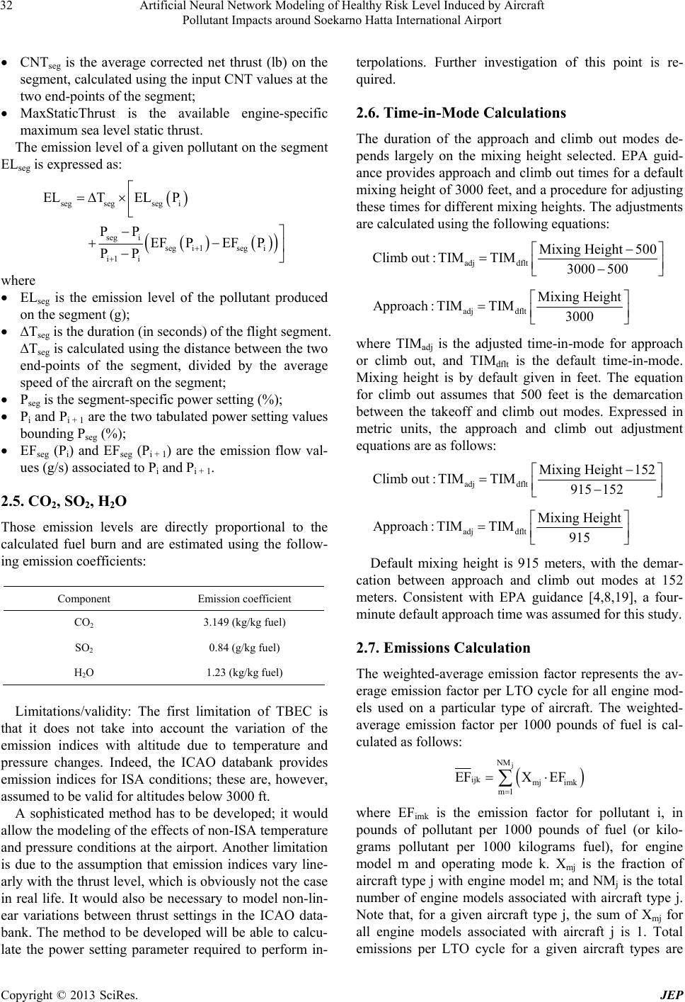

Artificial Neural Network Modeling of Healthy Risk Level Induced by Aircraft
Pollutant Impacts around Soekarno Hatta International Airport
32
 CNTseg is the average corrected net thrust (lb) on the
segment, calculated using the input CNT values at the
two end-points of the segment;
 MaxStaticThrust is the available engine-specific
maximum sea level static thrust.
The emission level of a given pollutant on the segment
ELseg is expressed as:

 

segsegsegi
seg i
segi1segi
i1 i
ELTEL P
PP
EF PEF P
PP 


 





where
 ELseg is the emission level of the pollutant produced
on the segment (g);
 ∆Tseg is the duration (in seconds) of the flight segment.
∆Tseg is calculated using the distance between the two
end-points of the segment, divided by the average
speed of the aircraft on the segment;
 Pseg is the segment-specific power setting (%);
 Pi and Pi + 1 are the two tabulated power setting values
bounding Pseg (%);
 EFseg (Pi) and EFseg (Pi + 1) are the emission flow val-
ues (g/s) associated to Pi and Pi + 1.
2.5. CO2, SO2, H2O
Those emission levels are directly proportional to the
calculated fuel burn and are estimated using the follow-
ing emission coefficients:
Component Emission coefficient
CO2 3.149 (kg/kg fuel)
SO2 0.84 (g/kg fuel)
H2O 1.23 (kg/kg fuel)
Limitations/validity: The first limitation of TBEC is
that it does not take into account the variation of the
emission indices with altitude due to temperature and
pressure changes. Indeed, the ICAO databank provides
emission indices for ISA conditions; these are, however,
assumed to be valid for altitudes below 3000 ft.
A sophisticated method has to be developed; it would
allow the modeling of the effects of non-ISA temperature
and pressure conditions at the airport. Another limitation
is due to the assumption that emission indices vary line-
arly with the thrust level, which is obviously not the case
in real life. It would also be necessary to model non-lin-
ear variations between thrust settings in the ICAO data-
bank. The method to be developed will be able to calcu-
late the power setting parameter required to perform in-
terpolations. Further investigation of this point is re-
quired.
2.6. Time-in-Mode Calculations
The duration of the approach and climb out modes de-
pends largely on the mixing height selected. EPA guid-
ance provides approach and climb out times for a default
mixing height of 3000 feet, and a procedure for adjusting
these times for different mixing heights. The adjustments
are calculated using the following equations:
adj dflt
Mixing Height500
TIM TIM3000 500 Climb out:




adj dflt
MixingH
Approa eight TIM TIM300 0 ch : 

where TIMadj is the adjusted time-in-mode for approach
or climb out, and TIMdflt is the default time-in-mode.
Mixing height is by default given in feet. The equation
for climb out assumes that 500 feet is the demarcation
between the takeoff and climb out modes. Expressed in
metric units, the approach and climb out adjustment
equations are as follows:
adj dflt
Mixing Height152
TIM TIM915 152 Climb out:




adj dflt
Mixing
Approac Height TIM TIM95 h: 1



Default mixing height is 915 meters, with the demar-
cation between approach and climb out modes at 152
meters. Consistent with EPA guidance [4,8,19], a four-
minute default approach time was assumed for this study.
2.7. Emissions Calculation
The weighted-average emission factor represents the av-
erage emission factor per LTO cycle for all engine mod-
els used on a particular type of aircraft. The weighted-
average emission factor per 1000 pounds of fuel is cal-
culated as follows:

j
NM
ijk mj imk
m1
EFXEF

 
where EFimk is the emission factor for pollutant i, in
pounds of pollutant per 1000 pounds of fuel (or kilo-
grams pollutant per 1000 kilograms fuel), for engine
model m and operating mode k. Xmj is the fraction of
aircraft type j with engine model m; and NMj is the total
number of engine models associated with aircraft type j.
Note that, for a given aircraft type j, the sum of Xmj for
all engine models associated with aircraft j is 1. Total
emissions per LTO cycle for a given aircraft types are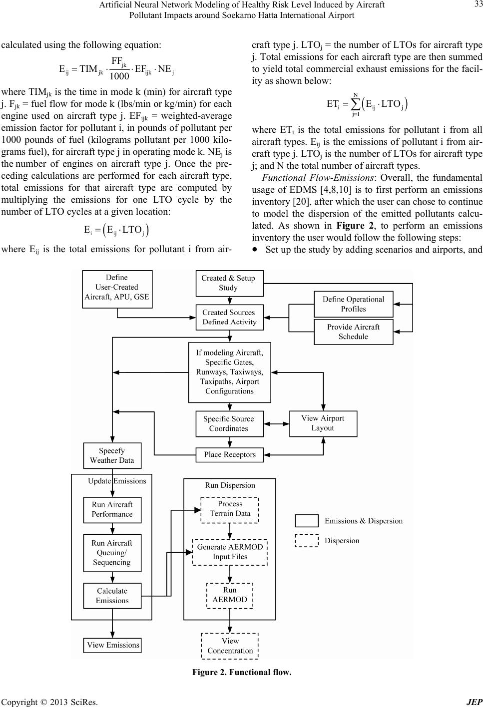

Artificial Neural Network Modeling of Healthy Risk Level Induced by Aircraft
Pollutant Impacts around Soekarno Hatta International Airport
33
craft type j. LTOj = the number of LTOs for aircraft type
j. Total emissions for each aircraft type are then summed
to yield total commercial exhaust emissions for the facil-
ity as shown below:
calculated using the following equation:
jk
ijjkijk j
FF
ETIMEFNE
1000

where TIMjk is the time in mode k (min) for aircraft type
j. Fjk = fuel flow for mode k (lbs/min or kg/min) for each
engine used on aircraft type j. EFijk = weighted-average
emission factor for pollutant i, in pounds of pollutant per
1000 pounds of fuel (kilograms pollutant per 1000 kilo-
grams fuel), for aircraft type j in operating mode k. NEj is
the number of engines on aircraft type j. Once the pre-
ceding calculations are performed for each aircraft type,
total emissions for that aircraft type are computed by
multiplying the emissions for one LTO cycle by the
number of LTO cycles at a given location:

iij
EELTO j
j

N
iij
j1
ETE LTO

 
where ETi is the total emissions for pollutant i from all
aircraft types. Eij is the emissions of pollutant i from air-
craft type j. LTOj is the number of LTOs for aircraft type
j; and N the total number of aircraft types.
Functional Flow-Emissions: Overall, the fundamental
usage of EDMS [4,8,10] is to first perform an emissions
inventory [20], after which the user can chose to continue
to model the dispersion of the emitted pollutants calcu-
lated. As shown in Figure 2, to perform an emissions
inventory the user would follow the following steps:
 Set up the study by adding scenarios and airports, and
where Eij is the total emissions for pollutant i from air-
Figure 2. Functional flow.

Artificial Neural Network Modeling of Healthy Risk Level Induced by Aircraft
Pollutant Impacts around Soekarno Hatta International Airport
34
choose which modeling options to use.
 Define all emissions sources, including operational
usage.
 Define the airport layout if sequence modeling was
selected.
 Select a weather option: annual average or hourly
(requires running AERMET).
 Select Update Emissions Inventory.
The simplest way to generate an emissions inventory
and obtain a course estimate of the total annual emissions
is to perform the first two steps, and use the ICAO/EPA
default times in mode along with the default operational
profiles, and the annual average weather from the EDMS
airports database [3,4,8,10,19,20]. Doing so would only
consider the total number of operations for the entire year
without regard to when those operations occurred. If a
more precise modeling of the aircraft taxi times using the
Sequencing module is desired (required if dispersion will
be performed), then the user must define the airport gates,
taxiways, runways, taxi paths (how the taxiways and
runways are used) and configurations (weather depend-
ent runway usage). The resulting emissions values can be
viewed by selecting Emissions Inventory on the View
menu. These results can be printed by selecting Print
under the File menu while viewing the emissions inven-
tory.
3. Artificial Neural Network Methodology
Artificial neural networks are a very simplified version
of real neural networks [21-24]. The human nervous sys-
tem consists of 1011 to 1012 nerve cells and is able to
carry out 1012 to 1013 “switching processes”—a complex-
ity that cannot be rebuilt technically. Nevertheless, it is
possible to understand the principles and to reconstruct a
few cells that simulate the most important processes. In
the year 1943, Warren McCulloch and Walter Pitts
showed in their paper “A logical calculus of the ideas
immanent in nervous activity” that even simple neural
networks are able to calculate any arithmetic or logical
function. 1957, Frank Rosenblatt et al. developed the
first successful neuro-computer, the so-called “Mark 1
perceptron”, which was able to recognize simple patterns.
Neural networks on the base of back-propagation were
developed in the early seventies and still are today the
most popular networks [21-24].
A neural network can be described as a “black box” to
which no interference takes place and whose concrete
behavior is invisible [22,23]. Summarized, there are three
principal tasks the network has to fulfill (Figure 3):
There are many types of ANN. Many new ones are
being developed (or at least variations of existing ones).
Networks based on supervised and unsupervised learning
[22-25].
Figure 3. The three principal tasks of a neuron.
Supervised Learning: The network is supplied with a
sequence of both input data and desired (target) output
data network is thus told precisely by a “teacher” what
should be emitted as output. The teacher can during the
learning phase “tell” the network how well it performs
(“reinforcement learning”) or what the correct behavior
would have been (“fully supervised learning”) [22-25].
Self-Organization or Unsupervised Learning: A
training scheme in which the network is given only input
data, network finds out about some of the properties of
the data set , learns to reflect these properties in its output.
E.g. the network learns some compressed representation
of the data. This type of learning presents a biologically
more plausible model of learning. What exactly these
properties are, that the network can learn to recognise,
depends on the particular network model and learning
method [24,25].
Networks based on Feedback and Feed-forward
connections: The following shows some types in each
category.
Unsupervised Learning.
Feedback Networks:
1) Binary Adaptive Resonance Theory (ART1)
2) Analog Adaptive Resonance Theory (ART2,
ART2a)
3) Discrete Hopfield (DH)
4) Continuous Hopfield (CH)
5) Discrete Bidirectional Associative Memory (BAM)
6) Kohonen Self-organizing Map/Topology-preserving
map (SOM/TPM)
Feedforward-only Networks:
1) Learning Matrix (LM)
2) Sparse Distributed Associative Memory (SDM)
3) Fuzzy Associative Memory (FAM)
4) Counterprogation (CPN)-Supervised Learning
5) Feedback Networks:
 Brain-State-in-a-Box (BSB)-Fuzzy Congitive Map
(FCM)
 Boltzmann Machine (BM)
 Backpropagation through time (BPTT)
6) Feedforward-only Networks:
 Perceptron-Ada line-Madaline
 Backpropagation (BP)-Artmap
 Learning Vector Quantization (LVQ)
 Probabilistic Neural Network (PNN)
 General Regression Neural Network (GRNN)
Methodology: Training, Testing and Validation Data-
set
In the ANN methodology, the sample data is often

Artificial Neural Network Modeling of Healthy Risk Level Induced by Aircraft
Pollutant Impacts around Soekarno Hatta International Airport
35
subdivided into training, validation, and test sets. The
distinctions among these subsets are crucial. Ripley [26]
defined the following:
1) Training set: A set of examples used for learning
that is to fit the parameters (weights) of the classifier.
2) Validation set: A set of examples used to tune the
parameters of a classifier, for example to choose the
number of hidden units in a neural network.
3) Test set: A set of examples used only to assess the
performance (generalization) of a fully specified classi-
fier.
Neural networks are the only tools that fulfill all char-
acteristics as shown in Table 1.
Method for measurement, prediction and assessment
of environmental problems such as aircraft pollutant
emissions has been carried out. The use of certain meth-
ods will require justification and reliability that must be
demonstrated and proven. Various methods have been
adopted for the assessment of aircraft annoyances.
The use of different and separate methodology causes
a wide variation in results and there are some lacks of
information. Assessment methods show different ap-
proaches with different levels of uncertainty as well. This
uncertainty factor has seen from the value of the index
that is different from any used method. Because of these
problem and the recurrently exists no research activity on
risk human impact from aircraft emissions near the air-
port, it propose in this research to develop the model of
aircraft impact by combining different inputs, in particu-
lar concentration of pollutants (Figure 4) using Artificial
Neural.
Network to determine the healthy risk of people around
Table 1. The advantages of neural networks.
Characteristics
Method Diffusive sampling
measurements
as input?
High accuracy
of results?
Ability to
incorporate the
most important
parameters?
Easy to handle?Short
computing time?
Update and
enhancement
possible?
Dispersion Modeling X
Interpolation X X X
Interpolation with add
variable X X X
Regression models X X X X
Neural networks X X X X X X
Summation and transfer function (processing element)
Figure 4. The suggested ANN model.

Artificial Neural Network Modeling of Healthy Risk Level Induced by Aircraft
Pollutant Impacts around Soekarno Hatta International Airport
36
the airport so we can manage the land use around the
airport based on the healthy risk level. But the questions
are how to combine pollutant and noise emission [15,16],
which method that would be reliable to use for quantify-
ing the pollutant and noise emissions, how about the ac-
curacy and the uncertainty of model that would be reli-
able, how about the balanced approach between eco-
nomic, operational and environmental capacities, how far
the zoning area of the pollutant and noise emission that
affecting the people around airport, and what do we have
as model to combine pollutant and noise emissions.
Based on the problem, it will be carried out the re-
search on how to develop model of aircraft pollutant and
noise emissions, which is the most suitable approach to
be used, both for the assessment of pollutant and noise
emissions and also the combination of those methods of
assessment. To validate the developed model, it applies
the measurement of noise and pollutant emissions at
Soekarno Hatta International Airport—Cengkareng Indo-
nesia.
The methodology will be used for assessing aircraft
pollutant in this research is the ICAO methodology be-
cause of emission factors used are based on engine certi-
fication data in the ICAO Engine Exhaust Emission Da-
tabank that contains data sets of thrust (engine perform-
ance), fuel flow and emissions of components CO, NOx
and SOx. Since ICAO has the approaches more widely
used by various countries so that the concept of balanced
approach will use for the assessment of Soekarno-Hatta
International airport to assess the level of pollutant and
noise emissions around airport with considering the fu-
ture prospects of aircraft technologies.
ANN modeling is a flexible method, which enables
one to recognize highly complex non-linear correlations
[22]. Statistical assumptions like normal distribution are
not necessary, which makes them easy to handle in prin-
ciple. The network can be trained with real measurement
data and updated with new measurements, enhancing its
quality and making it the ideal method for the purpose of
this research.
Data has been collected into two parts: Primary Data
and Secondary Data. The Primary data consisted in noise
and pollutant emissions measurement at Soekarno Hatta
International Airport. The Secondary Data consist of
Physical Data of airport, Air Traffic/Distribution of type
of flight (time of flight/day) for one year, Topography
Data and Weather Data. Emission and Dispersion of
Modeling System (EDMS) has been carried out with
concentration grid space 1 km2.
Input variable s:
The new model ANN is used 1 layer input data with
four input variables. Those input variables are noise level
in decibel (dB) unit and concentration of pollutant emis-
sions (CO, NOx, and SOx) in ug/m3 unit. Input element
was obtained from EDMS calculate using air traffic data
in the year 2009 and its extrapolation for 2012 at
Soekarno Hatta Airport. 70% of the input data set is pre-
sented to the network during training, so that the network
can be adjusted according to its error.
15% data are used to measure the network generaliza-
tion and to halt the network when generalization stops
improving. Remaining data performs testing of an inde-
pendent measure of network performance during and
after training. The training stops when gives a higher
accuracy value with minimum training and testing errors.
Processing variable:
In process layer, proposed model used 1 hidden layer
with 10 neurons which is the best architecture model
ANN that obtain from tool ANN after several times
process using sigmoid activation where the sigmoid ac-
tivation function is the best performances in ANN. It can
be described by the mathematical relationship


x
11 e

.
Weight and Bias values is shown in Tables 2 and 3.
Output variable:
One layer for output layer was used to determine the
healthy risk level as a target where the level has 5 healthy
risks level that effect from aircraft noise and pollutant.
The Levenberg-Marquadt (LM) training algorithm
outperformed in this research by training the high dimen-
sional data in 34 epochs with the time of 1 second. The
performance measures and outcome of the network are
depicted below.
Number of Epochs 34
Training (R) 0.97
Testing (R) 0.95
Validation (R) 0.95
Mean Squared Error Less than 1%
The error measures like Mean Squared Error (MSE)
are recorded. MSE is the mean of the squared error be-
tween the desired output and the actual output of the
neural network. The MSE is computed as follows.

2
PN
j0 iij 0ij
dy
MSE
N
P
 

where P is the number of output processing elements.
N: the number of exemplars in the training data set;
yij: the estimated network emissions output for exem-
plar i at processing element j;
dij the actual output for emissions exemplar i at proc-
essing element j. In this research the obtained MSE value
is less than 1% which was attained at 28th epoch. There
are 3 criteria based on ANN validation that choose to

Artificial Neural Network Modeling of Healthy Risk Level Induced by Aircraft
Pollutant Impacts around Soekarno Hatta International Airport
37
Table 2. Healthy risk level.
Pollutant Emissions
Risk Score Level
CO (µg/m3) NOx (µg/m3) SOx (µg/m3)
Noise (dB) Additional
and not necessary input
#5 Hazardous >200 >200 >200 >85
#4 Unhealthy 100 - 200 99.64 - 200 85.8 - 200 70 - 85
#3 Moderate 50 - 100 50 - 99.64 50 - 85.8 60 - 70
#2 Good 25 - 50 25 - 50 25 - 50 50 - 60
#1 Healthy <25 <25 <25 <50
Table 3. Network weights and bias values.
Weights Bias
Input Hidden (IW)
CO NOx SOx Noise:
additional index
Hidden Output
(LW) (b1) (b2)
w1 0.1407 −0.35259 2.2921 −1.1287 1.2221 b1 2.1849 1.2555
w2 −1.4491 −0.18607 −1.8873 −0.26701 1.1295 b2 2.0254
w3 1.3516 2.9137 0.27905 0.89349 2.3592 B3 −2.8272
w4 1.4867 −0.48544 −1.5046 −1.5885 −0.75403 b4 −1.1238
w5 −1.2303 −0.84468 1.1476 1.0959 −3.8315 b5 0.73
w6 0.93944 0.82249 −1.0546 2.368 −0.20789 b6 −2.4039
w7 −0.37134 0.88173 −0.88702 −1.3128 −1.1142 b7 −0.28432
w8 −0.18717 −1.8745 0.024024 5.5257 3.3151 b8 3.8534
w9 −0.8133 1.2728 0.49045 1.2881 1.0377 b9 −2.834
w10 1.4671 2.4003 0.22196 0.2502 −0.77638 b10 3.7339
validate the proposed of new model. Criteria 1 (Figure 5)
is based on performance, Criteria 2 (Figure 6) is based
on Regression R Value and Criteria 3 (Figure 7) is based
on networks output errors. All Criteria give a best result
of proposed ANN network. In Criteria 1, best validation
performance is achieved at epoch 28 from 34 epochs
(Mean Squared Error is 0.0093521). The correlation
(Criteria 2) between target and output is validated at R =
0.95756, means there is a close relation between target
and output. Criteria 3 show network output errors. The
range error value is close to zero (−0.4 - 0.6). According
to ANN Criteria it can be say that the proposed model is
valid. All the results are shown in below.
The example result of simulation for Soekarno Hatta
Airport, taking into account 2012 air traffic, is given in
the following table. Pollutants considered were CO, HC, Figure 5. Criteria 1.

Artificial Neural Network Modeling of Healthy Risk Level Induced by Aircraft
Pollutant Impacts around Soekarno Hatta International Airport
38
Figure 6. Criteria 2.
Figure 7. Criteria 3.
NOx and SOx.
ANN
calculation CO (t/y) HC (t/y) NOx (t/y) SOx (t/y)
Aircraft 3025261 137216 1640890 145823
It corresponds to an increase by 6% of pollutant emis-
sions a year since 2009.
4. Conclusions
Neural network model has been performed to assess en-
vironmental effects and impacts of air traffic on popula-
tions leaving around Soekarno Hatta International Air-
port-Cengkareng Indonesia. Assessment methods con-
sisting of statistical analysis, internal criteria of the neu-
ral network method proved the high quality of the model
outputs. ANN was used with the best architecture model
4-10-1. The suggested model has been validated by nu-
merical processing and experimental date. In Criteria 1,
best validation performance is achieved at epoch 28
(Mean Squared Error is less than 1%). The correlation
(Criteria 2) between target and output is validated at R =
96%. There is a close relation between target and outputs.
Criteria 3 show network output errors closed to zero. For
this developed model, concentration grid area was 1 km2.
The result map effect around this airport was a fine
structure to be considered on the area of 308 km2.
In addition, a sophisticated method has to be devel-
oped; it would allow the modeling of the effects of non-
ISA temperature and pressure conditions at the airport.
Particular assumptions concerning linearity variation of
emissions with the thrust level have to be avoided. Mod-
eling of non-linear variations of thrust settings has to be
improved. Further research is needed with the aim to
enlarge the scheme of the ANN model by increasing its
input variables and a refinement of the grid around air-
port. This is one of the major key defining environmental
capacities of an airport that should be applied by Indone-
sian airport authorities and international airports. These

Artificial Neural Network Modeling of Healthy Risk Level Induced by Aircraft
Pollutant Impacts around Soekarno Hatta International Airport
39
would institute policies to manage or reduce pollutant
emissions considering population and income growth to
be socially positive.
REFERENCES
[1] International Civil Aviation Organization (ICAO), “Air-
port Local Air Quality Guidance Manual,” 2007.
http://www.icao.int/icaonet/dcs/9889/9889_en.pdf
[2] International Civil Aviation Organization (ICAO), “En-
vironmental Report,” 2007.
http://www.icao.int/environmental-protection/.../ENV_Re
port_2010.pdf
[3] European Environmental Agency (EEA), “Emission In-
ventory Guidebook,” 2009.
http://www.eea.europa.eu/themes/air/emep-eea-air-pollut
ant-emission-inventory-guidebook/emep
[4] Federal Aviation Administration (FAA), “Office Envi-
ronment and Energy, Aviation & Emissions A Primer,”
2005.
http://www.faa.gov/regulations_policies/policy_guidance/
envir_policy/media/aeprimer.pdf
[5] M. Dameris, V. Grewe, I. Kohler, P. Sausen, C. Bruehl, J.
Grooss and B. Steil, “Impact of Aircraft NOx Emissions
on Tropospheric and Stratospheric Ozone, Part II: 3-D
Model Results,” Atmospheric Environment, Vol. 32, No.
18, 1998, pp. 3185-3199.
doi:10.1016/S1352-2310(97)00505-0
[6] B. E. Anderson, C. Gao and D. R. Blake, “Hydrocarbon
Emissions from a Modern Commercial Airliner,” Atmos-
pheric Environment, Vol. 40, No. 19, 2006, pp. 3601-
3612. doi:10.1016/j.atmosenv.2005.09.072
[7] J. S. Kurniawan and S. Khardi, “Comparison of Method-
ologies Estimating Emissions of Aircraft Pollutants, En-
vironmental Impact Assessment around Airports,” Envi-
ronmental Impact Assessment Review, Vol. 31, No. 3,
2011, pp. 240-252. doi:10.1016/j.eiar.2010.09.001
[8] Federal Aviation Administration (FAA), “Air Quality
Procedures for Civilian Airports and Air Force Bases,
Appendix D: Aircraft Emission Methodology,” 1997.
http://www.faa.gov/regulations_policies/policy_guidance/
envir_policy/airquality_handbook/media/Handbook.pdf
[9] M. Gauss, I. S. A. Isaksen, D. S. Lee and O. A. Sovde,
“Impact of Aircraft NOx Emissions on the Atmosphere—
Tradeoffs to Reduce the Impact,” Atmospheric Chemistry
and Physics, Vol. 5, 2005, pp. 12255-12311.
doi:10.5194/acpd-5-12255-2005
[10] Federal Aviation Administration (FAA), “Emission Dis-
persion Modeling System,” 2009.
http://www.faa.gov/about/office_org/headquarters_offices
/aep/models/
[11] International Civil Aviation Organization (ICAO), “In-
ternational Standards and Recommended Practices,” En-
vironmental Protection Annex 16, Volume II Aircraft En-
gine Emissions, 2nd Edition, ICAO, Montréal, 1993.
[12] International Civil Aviation Organization (ICAO), “Air-
craft-Operations-Flight-Procedures,” Doc-8168-Vol. 1,
5th Edition, ICAO, Montréal, 2006.
[13] International Civil Aviation Organization (ICAO), “An-
nex-16-Vol-2-3rd-Edition, Aircraft Engine Emissions,”
2008.
www.icao.int/environmental-protection/technology-stand
ards_FR.aspx
[14] J. G. J. Olivier, “Inventory of Aircraft Emissions: A Re-
view of Recent Literature,” Report No. 736 301 008, Na-
tional Institute of Public Health and Environmental Pro-
tection, Bilthoven, 1991
[15] S. Khardi, “Development of Innovative Optimized Flight
Paths of Aircraft Takeoffs Reducing Noise and Fuel Con-
sumption,” Acta Acustica United with Acustica, Vol. 97,
No. 1, 2011, pp. 148-154.
[16] S. Khardi and L. Abdallah, “Optimization Approaches of
Aircraft Flight Path Reducing Noise: Comparison of
Modeling Methods,” Applied Acoustics, Vol. 73, No. 4,
2012, pp. 291-301. doi:10.1016/j.apacoust.2011.06.012
[17] ALAQS, “Airport Local Air Quality Studies,” 2009.
http://www.isa-software.com/Alaqsstudy
[18] Sourdine II WP5, “Airport Noise and Emission Modeling
Methodology,” 2005.
http://www.sourdine.org/documents/public/SII_WP5_D5-
2_v10.pdf
[19] Environmental Protection Agency (EPA), “Evaluation of
Air Pollutant Emissions from Subsonic Commercial Jet
Aircraft,” 1999.
http://www.epa.gov/fedrgstr/EPA-AIR/2005/November/
Day-17/a22704.htm
[20] S. Baughcun, et al., “Scheduled Aircraft Emission Inven-
tories for 1992. Database Development and Analysis,”
NASA Contract Report No. 4700, NASA Langley Re-
search Centre, Washington DC, 1996.
[21] A. Cochocki and R. Unbehauen, “Neural Networks for
Optimization and Signal Processing,” John Wiley & Sons,
Inc., New York, 1993.
[22] M. Gevrey, I. Dimopoulos and S. Lek, “Review and
Comparison of Methods to Study the Contribution of
Variables in Artificial Neural Network Models,” Eco-
logical Modeling, Vol. 160, No. 3, 2003, pp. 249-264.
doi:10.1016/S0304-3800(02)00257-0
[23] P. D. Wasserman, “Advanced Methods in Neural Com-
puting,” John Wiley & Sons, Inc., New York, 1993.
[24] Z. H. Zhou, J. Wu and W. Tang, “Ensembling Neural
Networks: Many Could Be Better than All,” Artificial In-
telligence, Vol. 137, No. 1-2, 2002, pp. 239-263.
[25] H. White, “Artificial Neural Networks: Approximation
and Learning Theory,” Blackwell Publishers, Inc., Cam-
bridge, 1992.
[26] B. D. Ripley, “Pattern Recognition and Neural Net-
works,” Cambridge University Press, Cambridge, 1996.
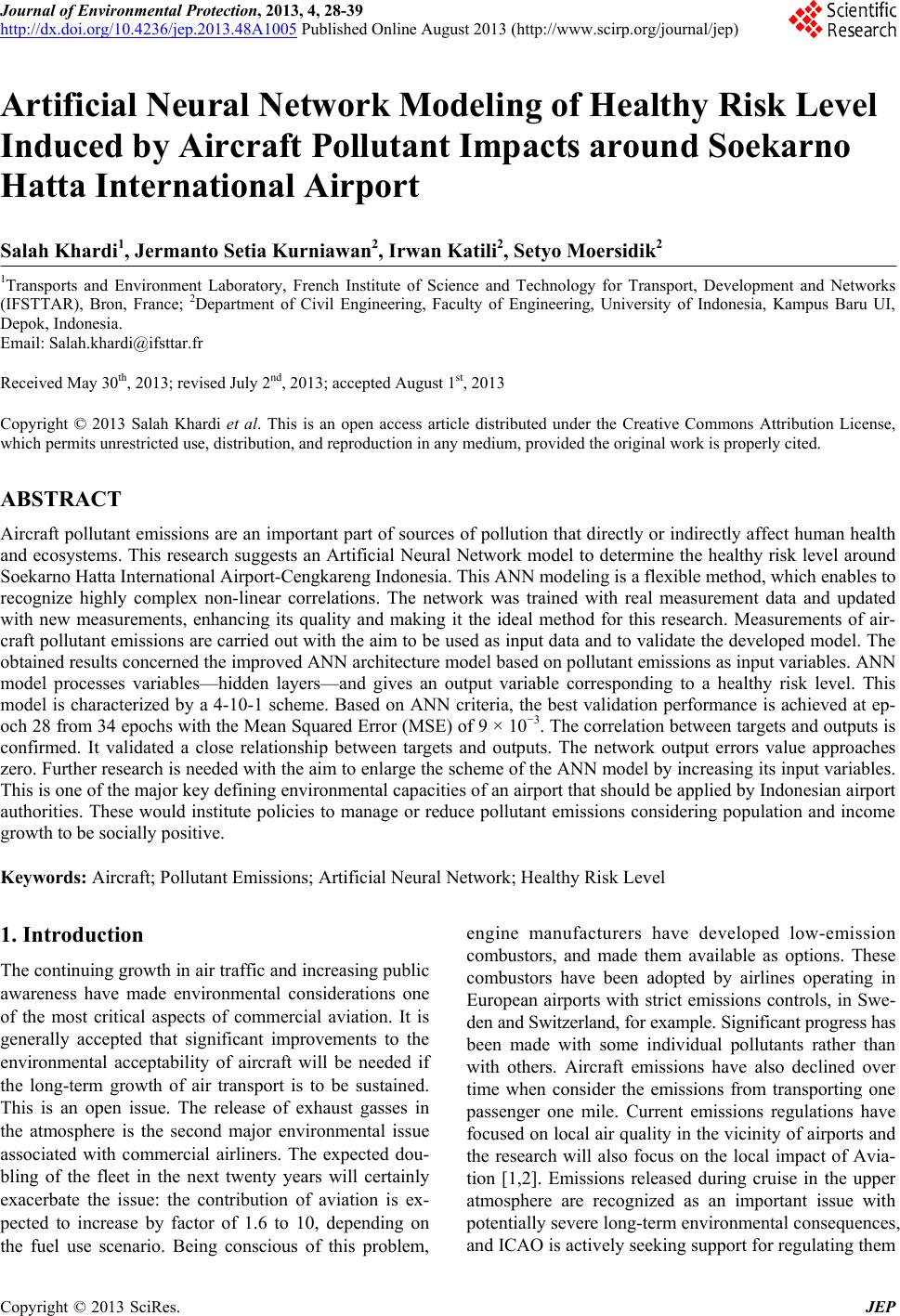