Journal of Environmental Protection, 2013, 4, 16-23
http://dx.doi.org/10.4236/jep.2013.48A1003 Published Online August 2013 (http://www.scirp.org/journal/jep)
An Analytical Air Pollution Model with Time Dependent
Eddy Diffusivity
Tiziano Tirabassi1*, Marco Túllio Vilhena2, Daniela Buske3, Gervásio Annes Degrazia4
1Institute of Atmospheric Sciences and Climate (ISAC), National Research Council (CNR), Bologna, Italy; 2Graduate Program in
Mechanical Engineering, Federal University of Rio Grande do Sul (UFRGS), Porto Alegre, Brazil; 3Department of Mathematics and
Statistics (IFM/DME), Federal University of Pelotas (UFPel), Pelotas, Brazil; 4Department of Physics, Federal University of Santa
Maria (UFSM), Santa Maria, Brazil.
Received April 30th, 2013; revised June 2nd, 2013; accepted July 5th, 2013
Copyright © 2013 Tiziano Tirabassi et al. This is an open access article distributed under the Creative Commons Attribution License,
which permits unrestricted use, distribution, and reproduction in any medium, provided the original work is properly cited.
ABSTRACT
Air pollution transport and dispersion in the atmospheric boundary layer are modeled by the advection-diffusion equa-
tion, that is, essentially, a statement of conservation of the suspended material in an incompressible flow. Many models
simulating air pollution dispersion are based upon the solution (numerical or analytical) of the advection-diffusion
equation assuming turbulence parameterization for realistic physical scenarios. We present the general time dependent
three-dimensional solution of the advection-diffusion equation considering a vertically inhomogeneous atmospheric
boundary layer for arbitrary vertical profiles of wind and eddy-diffusion coefficients. Numerical results and comparison
with experimental data are shown.
Keywords: Analytical Solution; Advection-Diffusion Equation; Air Pollution Modeling; Integral Transform;
Decomposition Method
1. Introduction
The processes governing the transport and diffusion of
pollutants present large variability and distinct forms, the
phenomenon is of such complexity that it would be im-
possible to describe it without the use of mathematical
models. Such models therefore constitute an indispensa-
ble technical instrument of air quality management.
The theoretical approach to the problem essentially
assumes different forms. In the K approach, diffusion is
considered, at a fixed point in space, proportional to the
local gradient of the concentration of the diffused mate-
rial. Consequently, it is fundamentally Eulerian since it
considers the motion of fluid within a spatially fixed
system of reference. They are based on the numerical
resolution, on a fixed spatial-temporal grid, of the equa-
tion of the mass conservation of the pollutant chemical
species, the so-said advection-diffusion equation (ADE).
However, in the last years, much progress has been
made in getting an analytical solution of steady state
ADE [1]. Recently, the literature presented analytical
general solutions of the ADE by the GILTT approach
(Generalized Integral Laplace Transform Technique)
whose main feature relies on the analytical solution of
transformed GITT (Generalized Integral Transform Tech-
nique) solutions by the Laplace Transform technique
[2,3]. This methodology has been largely applied in the
topic of simulations of pollutant dispersion in the At-
mospheric Boundary Layer (ABL) and is a general steady
state solution for any profiles of wind and eddy diffusiv-
ity. A new three-dimensional analytical solution is pre-
sented in this work for the prediction of pollutant disper-
sion in the ABL incorporating both the spatial and tem-
poral dependence of the eddy diffusivity.
To accomplish our objective, we solve the temporal
dependent three-dimensional advection-diffusion equa-
tion combining the Decomposition and GILTT ap-
proaches. So far, applying the idea of Decomposition
method [4,5], we reduce the ADE with temporal de-
pendence of the eddy diffusivity into a set of recursive
ADE’s with eddy diffusivity just depending on the spa-
tial variable z, which is then directly solved by the
GILTT method. We introduced an atmospheric boundary
Layer parameterisation with a time dependent vertical
eddy diffusivity coefficient and evaluated the performance
*Corresponding author.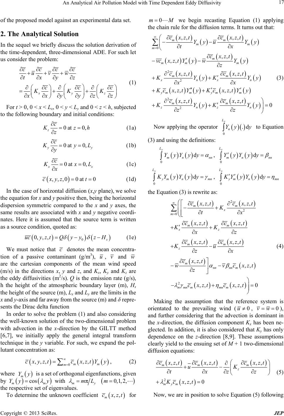

An Analytical Air Pollution Model with Time Dependent Eddy Diffusivity 17
of the proposed model against an experimental data set.
2. The Analytical Solution
In the sequel we briefly discuss the solution derivation of
the time-dependent, three-dimensional ADE. For such let
us consider the problem:
xyz
KKK
cccc
uvw
txyz
ccc
x
xy yz z
 


 

 



 
 
(1)
For t > 0, 0 < x < Lx, 0 < y < Ly and 0 < z < h, subjected
to the following boundary and initial conditions:
0at 0,
z
Kz
ch
z

 (1a)
0at 0,
y
y
K
L
y
cy 
 (1b)
0at 0,
x
x
K
L
x
cx 
 (1c)

,,,00at0xyzct

 (1d)
In the case of horizontal diffusion (x,y plane), we solve
the equation for x and y positive then, being the horizontal
dispersion symmetric compared to the x and y axes, the
same results are associated with x and y negative coordi-
nates. Here it is assumed that the source term is written
as a source condition, quoted as:
 
0
0,, ,

s
ucyz tQyyzH   
(1e)
We must notice that c denotes the mean concentra-
tion of a passive contaminant (g/m3), u, v and w
are the cartesian components of the mean wind speed
(m/s) in the directions x, y and z, and Kx, Ky and Kz are
the eddy diffusivities (m2/s). Q is the emission rate (g/s),
h the height of the atmospheric boundary layer (m), Hs
the height of the source (m), Lx and Ly are the limits in the
x and y-axis and far away from the source (m) and δ repre-
sents the Dirac delta function
In order to solve the problem (1) and also considering
the well-known solution of the two-dimensional problem
with advection in the x-direction by the GILTT method
[6,7], we initially apply the general integral transform
technique in the y variable. For such, we expand the pol-
lutant concentration as:
 
0
,,, ,,
mm
m
cxyztc xztYy





, (2)
where is a set of orthogonal eigenfunctions, given
by mm Yy with

m
Yy

cos

y  π
my
mL


the respective set of eigenvalues.

0,1,2,m
To determine the unknown coefficient

,,
m
cxzt

M
for
0m

 we begin recasting Equation (1) applying
the chain rule for the diffusion terms. It turns out that:

 

  

  
 

  
0
2
2
2
2
,, ,,
,,
,,
,, ,,
,, ,,
,,,, 0
mm
mm
m
m
mm m
mm
xnxn
ymm ymm
mm
znzn
cxztcxzt
Yy uYy
tx
cxzt
vc xztY ywY y
z
c xztc xzt
KYyKYy
x x
Kc xztY yKcxztY y
cxztcxzt
KYyKYy
zz


 









 
 







 

(3)
Now applying the operator to Equation
(3) and using the definitions:

0
.d
y
L
n
Yy y

 
0
d
y
L
mn
YyYyy nn


,
 
0
d
y
L
mn
YyYyy nn



 
0
d
y
L
y
mn
KYyY yymn


,
 
0
d
y
L
y
mn
KYyY yymn

 

the Equation (3) is rewrite as:


 
 
 
2,, ,, 0
mm nm mnm
cx ztcxzt  


2
2
0
,, ,,
,, ,,
,, ,,
,, ,,
mm
x
m
mm
xz
mm
z
m
nnnn m
cxzt cxzt
K
tx
cxzt cxzt
KK
xz
cxztcxzt
Ku
zx
cxzt
wvcxzt
z



























(4)
Making the assumption that the reference system is
orientated to the prevailing wind (0u, 0vw

),
and further considering that the advection is dominant in
the x-direction, the diffusion component Kx has been ne-
glected. In addition, it is also considered that Ky has only
dependence on the z-direction [8,9]. These assumptions
clearly yield to the ensuing set of M + 1 two-dimensional
diffusion equations:





2
,,,,,,
,, 0
mm m
z
mym
cxztcxztcxzt
uK
txzz
Kc xzt 
  






(5)
Now, we are in position to solve Equation (5) following

An Analytical Air Pollution Model with Time Dependent Eddy Diffusivity
18
the idea of the Decomposition method [4,5]. In fact to
construct the solution, firstly it is considered that the
time-dependent eddy diffusivity is written like:
 
,,
zz z
K
ztkztK z
(6)
where

z
K
z is the time averaged eddy diffusivity. By
this assumption the Equation (5) reads like:
 
  
 
2
,, ,,
,, ,,
,,
,
mm
m
zmy
m
z
cxztcxzt
u
tx
cxzt
m
K
zKc
zz
cxzt
kzt
zz




 





 




xzt (7)
According the idea of the Decomposition method, we
consider that the solution of Equation (7) has the form:

,
0
,,,,
J
mmj
j
c xztcxzt



(8)
Now replacing Equation (8) in Equation (7), from the
resulting equation we are able to construct the recursive
set of advective-diffusive equations:
 



 

  
,0 ,0,0
2
,0
,1 ,1,1
2
,1 1
,, ,
2
,, ,,,,
,, 0
,, ,,,,
,, ,,
,, ,,,,
mm m
z
mym
mm m
z
mym
mJ mJmJ
z
my
cxzt cxztcxzt
uKz
txzz
Kc xzt
cxzt cxztcxzt
uKz
txzz
KcxztS xzt
cxzt cxztcxzt
uKz
txzz
K



  






  






  








,,, ,, mJ J
cxztS xzt

























(9)
where we have the following notation for the term :
J
S
  
,1 ,,
,, ,
for 1:
mJ
Jz
cxzt
Sxzt kzt
zz
lJ

 





(10)
We must recall that this procedure is not unique. We
justify our choice in order because this procedure allows
us to take advantage from the fact that the resulting re-
cursive system problem can be straightly analytically
solved by the GILTT approach [6,7,10]. Further we have
to notice that the time dependence of the eddy diffusivity
in the proposed solution is governed by the source term.
It is relevant underline that the first equation of recursive
system problems satisfies the boundary conditions
(Equations (1a-e)) meanwhile the remaining equations
satisfy the homogeneous boundary condition. Once the
set of problems (9) is solved by the GILTT method, the
solution of Equation (1) is well determined. It is impor-
tant to remark that we may control the accuracy of the
results by a proper choice of the number of terms in the
series solution summation.
3. Model Evaluation against Experimental
Data
The performance of the proposed model is evaluated
against the experimental Copenhagen [11,12] data set. In
the Copenhagen experiment the tracer SF6 was released
without buoyancy from a tower at a height of 115 m, and
collected at the ground-level positions at a maximum of
three crosswind arcs of tracer sampling units. The sam-
pling units were positioned, at the ground level, 2 - 6 km
from the point of release. The site was mainly residential
with a roughness length of 0.6 m. The meteorological
conditions during the dispersion experiments ranged
from moderately unstable to convective. We used the
values of the maximum concentration on every cross-
wind arc normalized with the tracer release rate from
[11]. Generally, the distributed data set contains hourly
mean values of concentrations and meteorological data.
However, in this model the validation is performed to
show the time dependence of eddy diffusivity using data
with a greater time resolution, kindly made available by
Gryning and described in [13]. In particular, we used 10
minutes averaged values for meteorological data in Ta-
bles 1-3 while Table 4 reported hourly mean values of
Table 1. Friction velocity (u* (m/s)) for different time steps.
Each interval corresponds to 10 min.
t/Run1 2 3 4 5 7 8 9
1 0.360.68 0.46 0.56 0.58 0.48 0.650.72
2 0.370.67 0.45 0.51 0.52 0.48 0.790.73
3 0.400.81 0.47 0.37 0.51 0.57 0.670.60
4 0.430.68 0.39 0.44 0.58 0.62 0.670.59
5 0.350.75 0.39 0.48 0.59 0.53 0.680.65
6 0.340.74 0.40 0.48 0.52 0.65 0.650.71
7 0.420.76 0.40 0.39 0.52 0.63 0.680.73
8 0.430.82 0.41 0.40 0.45 0.65 0.670.73
9 0.400.76 0.31 0.39 0.44 0.66 0.730.73
10 0.37 0.73 0.340.39 0.44 0.62 0.73 0.66
11 0.35 0.69 0.390.39 0.44 0.52 0.75 0.67
12 0.36 0.66 0.400.39 0.43 0.62 0.69 0.74

An Analytical Air Pollution Model with Time Dependent Eddy Diffusivity 19
Table 2. Convective velocity (w* (m/s)) for different time
steps. Each interval corresponds to 10 min.
t/Run 1 2 3 4 5 7 8 9
1 2.07 2.04 1.21 1.32 0.93 1.93 1.99 1.35
2 2.22 1.85 1.10 1.45 1.10 1.86 2.27 1.63
3 1.56 2.02 1.40 1.29 0.90 2.37 2.35 1.77
4 2.11 2.11 1.18 1.37 0.82 2.15 2.32 1.43
5 1.81 2.15 1.09 1.15 1.05 1.57 2.42 1.31
6 1.67 1.89 1.37 1.10 1.02 2.67 2.07 1.47
7 1.98 2.39 1.29 0.89 1.02 2.37 2.49 1.51
8 2.18 2.26 1.48 0.85 0.89 2.62 2.35 1.63
9 1.56 2.25 0.92 0.77 0.76 2.87 2.24 1.74
10 2.29 1.69 1.38 0.770.76 2.15 2.31 1.59
11 1.88 2.28 1.18 0.770.76 1.45 2.54 1.82
12 2.00 1.54 1.37 0.770.60 2.08 2.57 2.03
Table 3. Monin-Obukhov length (m) for the different runs
and time steps. Each time step corresponds to 10 min.
t/Run 1 2 3 4 5 7 8 9
1 −26 −178 −152 −75−492 −71 −71 −793
2 −23 −227 −194 −42−215 −80 −85 −471
3 −83 −311 −106 −23−368 −64 −47 −202
4 −42 −160 −101 −32−735 −111 −49−366
5 −36 −203 −129 −71−366 −177 −45−633
6 −42 −286 −70 −80 −273 −67 −63 −588
7 −47 −155 −83 −83 −273 −87 −41 −593
8 −38 −228 −60 −101 −262 −71 −47 −471
9 −83 −184 −106 −129 −395 −56 −70 −389
10 −21 −389 −42 −129 −395 −111 −64 −375
11 −32 −133 −101 −129 −395 −215 −52 −262
12 −29 −375 −70 −129 −759 −123 −39 −252
Table 4. Boundary layer height for the differe nt runs.
Run 1 2 3 4 5 7 8 9
h (m) 1980 1920 1120 390820 1850 8102090
boundary layer height.
Boundary Layer Parameterization
The reliability of the analytical solution of the advection-
diffusion equation depends on the choice of the atmos-
pheric boundary Layer parameterization. In terms of the
convective scaling parameters the vertical eddy diffusiv-
ity can be formulated as [14]:
11
48
33
*
0.2211 e0.0003e
zz
hh
z
Kzz
whh h
 

 
 

 


 
 


(11)
The above formulation of the vertical eddy diffusivity
varies in time through the time variation of the vertical
convective velocity w* and the height of the ABL h. In
Figure 1 we show the graphic displaying the vertical
eddy diffusivity Kz as a sectional function of time for the
Copenhagen data set.
For the lateral diffusion we used [14]:

π
16
v
y
mv
v
K
f
q

 (12)
with

2/3 2/3
22
*
2/3
0.98 v
v
v
mv
czw
qh
f








 ; 4.16
v
z
qh ;


mv
f

0.16 and
1/2
22/3
1/3 10.7
zz
hL



5



 







. More, k is

the von Karman constant (k = 0.4), L is the Monin-
Obukhov length, v

is the Eulerian standard deviation
of the longitudinal turbulent velocity, v is the stability
function,
q


is the non-dimensional molecular dissipa-
tion rate function,


mv
f
is the peak wavelength of the
turbulent velocity spectra.
Figure 1. Vertical eddy diffusivity profile (Kz) in function of
time for the Copenhagen experime ntal runs.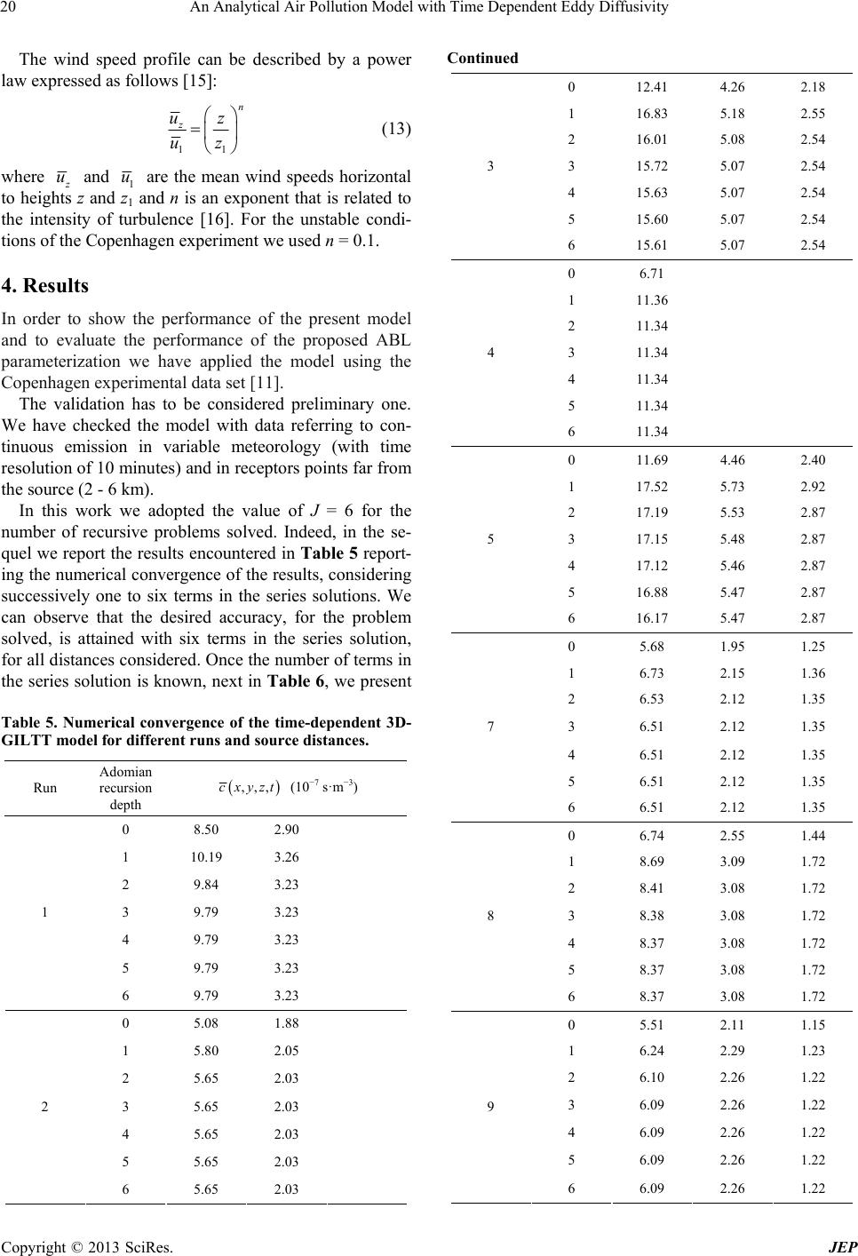

An Analytical Air Pollution Model with Time Dependent Eddy Diffusivity
20
The wind speed profile can be described by a power
law expressed as follows [15]:
11
n
z
uz
uz



(13)
where
z
u and 1 u are the mean wind speeds horizontal
to heights z and z1 and n is an exponent that is related to
the intensity of turbulence [16]. For the unstable condi-
tions of the Copenhagen experiment we used n = 0.1.
4. Results
In order to show the performance of the present model
and to evaluate the performance of the proposed ABL
parameterization we have applied the model using the
Copenhagen experimental data set [11].
The validation has to be considered preliminary one.
We have checked the model with data referring to con-
tinuous emission in variable meteorology (with time
resolution of 10 minutes) and in receptors points far from
the source (2 - 6 km).
In this work we adopted the value of J = 6 for the
number of recursive problems solved. Indeed, in the se-
quel we report the results encountered in Table 5 report-
ing the numerical convergence of the results, considering
successively one to six terms in the series solutions. We
can observe that the desired accuracy, for the problem
solved, is attained with six terms in the series solution,
for all distances considered. Once the number of terms in
the series solution is known, next in Table 6, we present
Table 5. Numerical convergence of the time-dependent 3D-
GILTT model for different runs and source distances.
Run
Adomian
recursion
depth

,,,cxyzt
Continued
0 12.41 4.26 2.18
1 16.83 5.18 2.55
2 16.01 5.08 2.54
3 15.72 5.07 2.54
4 15.63 5.07 2.54
5 15.60 5.07 2.54
3
6 15.61 5.07 2.54
0 6.71
1 11.36
2 11.34
3 11.34
4 11.34
5 11.34
4
6 11.34
0 11.69 4.46 2.40
1 17.52 5.73 2.92
2 17.19 5.53 2.87
3 17.15 5.48 2.87
4 17.12 5.46 2.87
5 16.88 5.47 2.87
5
6 16.17 5.47 2.87
0 5.68 1.95 1.25
1 6.73 2.15 1.36
2 6.53 2.12 1.35
3 6.51 2.12 1.35
4 6.51 2.12 1.35
5 6.51 2.12 1.35
7
6 6.51 2.12 1.35
0 6.74 2.55 1.44
1 8.69 3.09 1.72
2 8.41 3.08 1.72
3 8.38 3.08 1.72
4 8.37 3.08 1.72
5 8.37 3.08 1.72
8
6 8.37 3.08 1.72
0 5.51 2.11 1.15
1 6.24 2.29 1.23
2 6.10 2.26 1.22
3 6.09 2.26 1.22
4 6.09 2.26 1.22
5 6.09 2.26 1.22
9
6 6.09 2.26 1.22

(10−7 s·m−3)
0 8.50 2.90
1 10.19 3.26
2 9.84 3.23
3 9.79 3.23
4 9.79 3.23
5 9.79 3.23
1
6 9.79 3.23
0 5.08 1.88
1 5.80 2.05
2 5.65 2.03
3 5.65 2.03
4 5.65 2.03
5 5.65 2.03
2
6 5.65 2.03

An Analytical Air Pollution Model with Time Dependent Eddy Diffusivity 21
Table 6. Observed and predicted concentrations data for
different runs (Copenhagen experiment) at various source
distances. The concentration is divided by the emission rate
Q.
Run Distance (m)
Observed
(10−7 s·m−3)
Predictions
(10−7 s·m−3)
1 1900 10.5 9.79
1 3700 2.14 3.23
2 2100 9.85 5.65
2 4200 2.83 2.03
3 1900 16.33 15.61
3 3700 7.95 5.07
3 5400 3.76 2.54
4 4000 15.71 11.34
5 2100 12.11 16.17
5 4200 7.24 5.47
5 6100 4.75 2.87
7 2000 9.48 6.51
7 4100 2.62 2.12
7 5300 1.15 1.35
8 1900 9.76 8.37
8 3600 2.64 3.08
8 5300 0.98 1.72
9 2100 8.52 6.09
9 4200 2.66 2.26
9 6000 1.98 1.22
numerical comparisons of the 3D-GILTT results against
experimental data.
In Figure 2 the scatter diagram of model results
against experimental data is presented and it can be ob-
served that the present models in good agreement with
experimental data.
In Table 7 some well-known statistical indices of
models performances are reported. They are suggested
and discussed in Chang and Hanna [17] and defined in
the following way:

2
NMSE op p CC CC o ,


FA2data for which0.52
po
CC,

COR oo p po CCCC p

  ,

FB 0.5
op op
CC CC ,

Figure 2. Observed (Co) and predicted (Cp) scatter plot.
Data between dotted lines corre spond to


0.5,2
op
CC

.
Table 7. Statistical indices of model performances.
Recursion
depth NMSECOR FA2 FB FS
0 0.30 0.90 0.95 0.36 0.35
1 0.12 0.91 1.00 0.11 −0.03
2 0.12 0.91 1.00 0.14 0.01
3 0.12 0.91 1.00 0.14 0.02
4 0.12 0.91 1.00 0.14 0.02
5 0.12 0.91 1.00 0.15 0.03
6 0.11 0.92 1.00 0.15 0.05
where NMSE is the normalized mean square error, COR
the correlation coefficient, FA2 is the fraction of data (%,
normalized to 1), FB the fractional bias, FS the fractional
standard deviations. Subscripts o and p refer to observed
and predicted quantities, respectively,  is the standard
deviation, C the concentration and the overbar indicates
an averaged value. The statistical index FB says if the
predicted quantities underestimate or overestimate the
observed ones. FA2 is the fraction of Co values (normal-
ized to 1) within a factor two of corresponding Cp values.
The statistical index NMSE represents the model values
dispersion in respect to data dispersion. The best results
are expected to have values near zero for the indices
NMSE, FB and FS, and near one in the indices COR and
FA2. So far, considering the statistical indices in Table 7
we can consider good the performance of the solution
with the presented ABL parameterization.

FS 0.5
op op

    ,

An Analytical Air Pollution Model with Time Dependent Eddy Diffusivity
22
5. Conclusions
In recent years, it was presented in the literature, for the
first time, a steady-state analytical solution for the advec-
tion-diffusion equation considering a vertically inhomo-
geneous PBL (with any restriction about the eddy diffu-
sivity coefficients and wind speed profiles) based on the
GILTT approach (Generalized Integral Laplace Trans-
form Technique) [2,3]. Here we present a three-dimen-
sional time-dependent solution with time-dependent ver-
tical eddy diffusivity profiles that can be used in a time
evolving turbulent boundary layer. Moreover, with the
assumed ABL parameterization the model can be applied
routinely using as input simple ground-level meteoro-
logical data acquired by an automatic network. Prelimi-
nary model performances evaluation confirms the reli-
ability of the model results.
We also underline the hierarchical character of this
methodology, in the sense that the solution of the three-
dimensional ADE problem is obtained from the solution
of two-dimensional ones. Furthermore, this hierarchical
character also prevails for problems with eddy diffusivity
depending on time. In fact, for such problem the solution
again attained from the solution of a set of problems with
eddy diffusivity depending only on the vertical variable,
having the main feature that the sources terms carry the
time-dependency information of the eddy diffusivity.
Therefore, from the previous discussion, we are confi-
dent that we have paved the road to construct a more
realistic analytical solution for this kind of problem by
now assuming a time dependency on the wind field too.
We shall focus our future attention in this direction.
6. Acknowledgements
The authors thank CNPq (Conselho Nacional de Desen-
volvimento Científico e Tecnológico) and FAPERGS
(Fundação de Amparo à Pesquisa do Estado do Rio
Grande do Sul) for the partial financial support of this
work.
REFERENCES
[1] T. Tirabassi, “Operational Advanced Air Pollution Mod-
elling,” Pure and Applied Geophysics, Vol. 160, No. 1-2,
2003, pp. 5-16. doi:10.1007/s00024-003-8762-y
[2] D. Buske, M. T. Vilhena, B. Bodmann and T. Tirabassi,
“Analytical Model for Air Pollution in the Atmospheric
Boundary Layer,” In: M. Khare, Ed., Air Pollution, Vol. 1,
InTech, Rijeka, 2012, pp. 39-58.
[3] D. M. Moreira, M. T. Vilhena, D. Buske and T. Tirabassi,
“The State-of-Art of the GILTT Method to Simulate Pol-
lutant Dispersion in the Atmosphere,” Atmospheric Re-
search, Vol. 92, No. 1, 2009, pp. 1-17.
doi:10.1016/j.atmosres.2008.07.004
[4] G. Adomian, “A New Approach to Nonlinear Partial Dif-
ferential Equations,” Journal of Mathematical Analysis
and Applications, Vol. 102, No. 2, 1984, pp. 420-434.
doi:10.1016/0022-247X(84)90182-3
[5] G. Adomian, “A Review of the Decomposition Method in
Applied Mathematics,” Journal of Mathematical Analysis
and Applications, Vol. 135, No. 2, 1988, pp. 501-544.
doi:10.1016/0022-247X(88)90170-9
[6] S. Wortmann, M. T. Vilhena, D. M. Moreira and D.
Buske, “A New Analytical Approach to Simulate the Pol-
lutant Dispersion in the PBL,” Atmospheric Environment,
Vol. 39, No. 12, 2005, pp. 2171-2178.
doi:10.1016/j.atmosenv.2005.01.003
[7] D. M. Moreira, M. T. Vilhena, T. Tirabassi, D. Buske and
R. Cotta, “Near Source Atmospheric Pollutant Dispersion
Using the New GILTT Method,” Atmospheric Environ-
ment, Vol. 39, No. 34, 2005, pp. 6290-6295.
doi:10.1016/j.atmosenv.2005.07.008
[8] J. C. Kaimal, J. C. Wyngaard, et al., “Turbulence Struc-
ture in the Convective Boundary Layer,” Journal of the
Atmospheric Sciences, Vol. 33, No. 11, 1976, pp. 2152-
2169.
doi:10.1175/1520-0469(1976)033<2152:TSITCB>2.0.CO
;2
[9] S. J. Caughey and S. G. Palmer, “Some Aspects of Tur-
bulence Structure through the Depth of the Convective
Boundary Layer,” Quarterly Journal of the Royal Mete-
orological Society, Vol. 105, No. 446, 1979, pp. 811-827.
doi:10.1002/qj.49710544606
[10] D. M. Moreira, M. T. Vilhena, D. Buske and T. Tirabassi,
“The GILTT Solution of the Advection-Diffusion Equa-
tion for an Inhomogeneous and Nonstationary PBL,”
Atmospheric Environment, Vol. 40, No. 17, 2006, pp.
3186-3194. doi:10.1016/j.atmosenv.2006.01.035
[11] S. E. Gryning and E. Lyck, “Atmospheric Dispersion
from Elevated Source in an Urban Area: Comparison
between Tracer Experiments and Model Calculations,”
Journal of Climate and Applied Meteorology, Vol. 23, No.
4, 1984, pp. 651-654.
doi:10.1175/1520-0450(1984)023<0651:ADFESI>2.0.C
O;2
[12] S. E. Gryning, A. A. M. Holtslag, J. S. Irwin and B.
Siversten, “Applied Dispersion Modelling Based on Me-
teorological Scaling Parameters,” Atmospheric Environ-
ment, Vol. 21, No. 1, 1987, pp. 79-89.
doi:10.1016/0004-6981(87)90273-3
[13] T. Tirabassi and U. Rizza, “Boundary Layer Parameteri-
zation for a Non-Gaussian Puff Model,” Journal of Ap-
plied Meteorology, Vol. 36, No. 8, 1997, pp. 1031-1037.
doi:10.1175/1520-0450(1997)036<1031:BLPFAN>2.0.C
O;2
[14] G. A. Degrazia, H. F. Campos Velho and J. C. Carvalho,
“Non-Local Exchange Coefficients for the Convective
Boundary Layer Derived from Spectral Properties,” Con-
tributions to Atmospheric Physics, Vol. 70, No. 1, 1997,
pp. 57-64.
[15] H. A. Panofsky and J. A. Dutton, “Atmospheric Turbu-
lence,” John Wiley & Sons, New York, 1984.
[16] J. S. Irwin, “A Theoretical Variation of the Wind Profile

An Analytical Air Pollution Model with Time Dependent Eddy Diffusivity
23
Power-Low Exponent as a Function of Surface Rough-
ness and Stability,” Atmospheric Environment, Vol. 13,
No. 1, 1979, pp. 191-194.
doi:10.1016/0004-6981(79)90260-9
[17] J. C. Chang and S. R. Hanna, “Air Quality Model Per-
formance Evaluation,” Meteorology and Atmospheric
Physics, Vol. 87, No. 1-3, 2004, pp. 167-196.
doi:10.1007/s00703-003-0070-7