 Journal of Modern Physics, 2013, 4, 1013-1021 http://dx.doi.org/10.4236/jmp.2013.47136 Published Online July 2013 (http://www.scirp.org/journal/jmp) Dynamics Behaviors of a Laser Produced Plasma: Theoretical Approach L. R. Manea1, C. Nejneru2, D. Mătăsaru3, C. I. Axinte2, M. Agop4,5 1Faculty of Textile, Leather Engineering and Industrial Management, “Gheorghe Asachi” Technical University of Iasi, Iasi, Romania 2Faculty of Materials Science and Engineering, “Gheorghe Asachi” Technical University of Iasi, Iași, Romania 3Department of Electronics and Telecommunication, “Gheorghe Asachi” Technical University of Iasi, Iași, Romania 4Lasers, Atoms and Molecules Physics Laboratory, University of Science and Technology, Lille, France 5Physics Department, “Gheorghe Asachi” Technical University of Iasi, Iasi, Romania Email: m.agop@yahoo.com Received April 24, 2013; revised May 26, 2013; accepted June 24, 2013 Copyright © 2013 L. R. Manea et al. This is an open access article distributed under the Creative Commons Attribution License, which permits unrestricted use, distribution, and reproduction in any medium, provided the original work is properly cited. ABSTRACT Assuming that plasma particles are moving on continuous and non-differentiable curves, some dynamic properties in plasma ablation are analyzed via scale-relativity theory: the splitting of plasma plume, multi-peak structures, at various distances from the target surface and plasma oscillations through self-similarity. Our theoretical results are in good agreement with the experimental ones. Keywords: Plasma Ablation; Fractal Curves; Plume Splitting; Plasma Oscillations 1. Introduction The interaction of high-power laser radiation with target materials is a topic of current interest in various fields such as material-processing, plasma physics, analytical sciences, etc. [1,2]. Laser ablation implies a series of complex phenomena: interaction of laser radiation with a solid target [3], laser beam absorption in ablation plume [4], hydrodynamics and electrical processes in the gener- ated transient plasma [5,6], etc. Correspondingly, theoretical models describing the dynamics related to these complex phenomena become sophisticated and ambiguous [1,2]. However, the situa- tion can be standardized taking into account that the ele- mentary processes induced by laser-matter interaction impose various temporal resolution scales [7,8], and that the pattern evolution imposes different degrees of free- dom e.g.: from one, at the initial stages, to three at the final stages of the patterns induced by the laser-produced plasma [9]. In the present paper various theoretical as- pects of a laser-ablation plasma dynamics (generation of two plasma structures, multi-peak structure for various distances from the target surface, plasma-ablation oscil- lations through self-similarity, etc.) were analyzed using the SR theory. 2. Hallmarks of Non-Differentiability For developing our theoretical model, we take into ac- count that, in plasma-ablation, deterministic chaos arises in association with spatio-temporal structures emergence. For temporal scales that are large with respect to the in- verse of the highest Lyapunov exponent, the determinis- tic trajectories can be replaced by collections of potential trajectories and the concept of definite positions by that of probability density. This concept was introduced in the framework of the scale relativity (SR) theory [10-12], which states that the particles movement takes place on continuous but non-differentiable curves (fractal curves). Subsequently, all physical phenomena become dependent not only on the spatio-temporal coordinates but also on the spatio-temporal scales. Thus the non-differentiability become a fundamental characteristic of the plasma-abla- tion dynamics. Non-differentiability implies the following [10-17]: 1) A continuous and non-differentiable curve (or al- most nowhere differentiable) is explicitly scale depend- ent. Moreover, its length tends to infinity, when the scale interval tends to zero. Consequently, according to Man- delbrot’s concept, a continuous and non-differentiable space will be a fractal space [18]; C opyright © 2013 SciRes. JMP 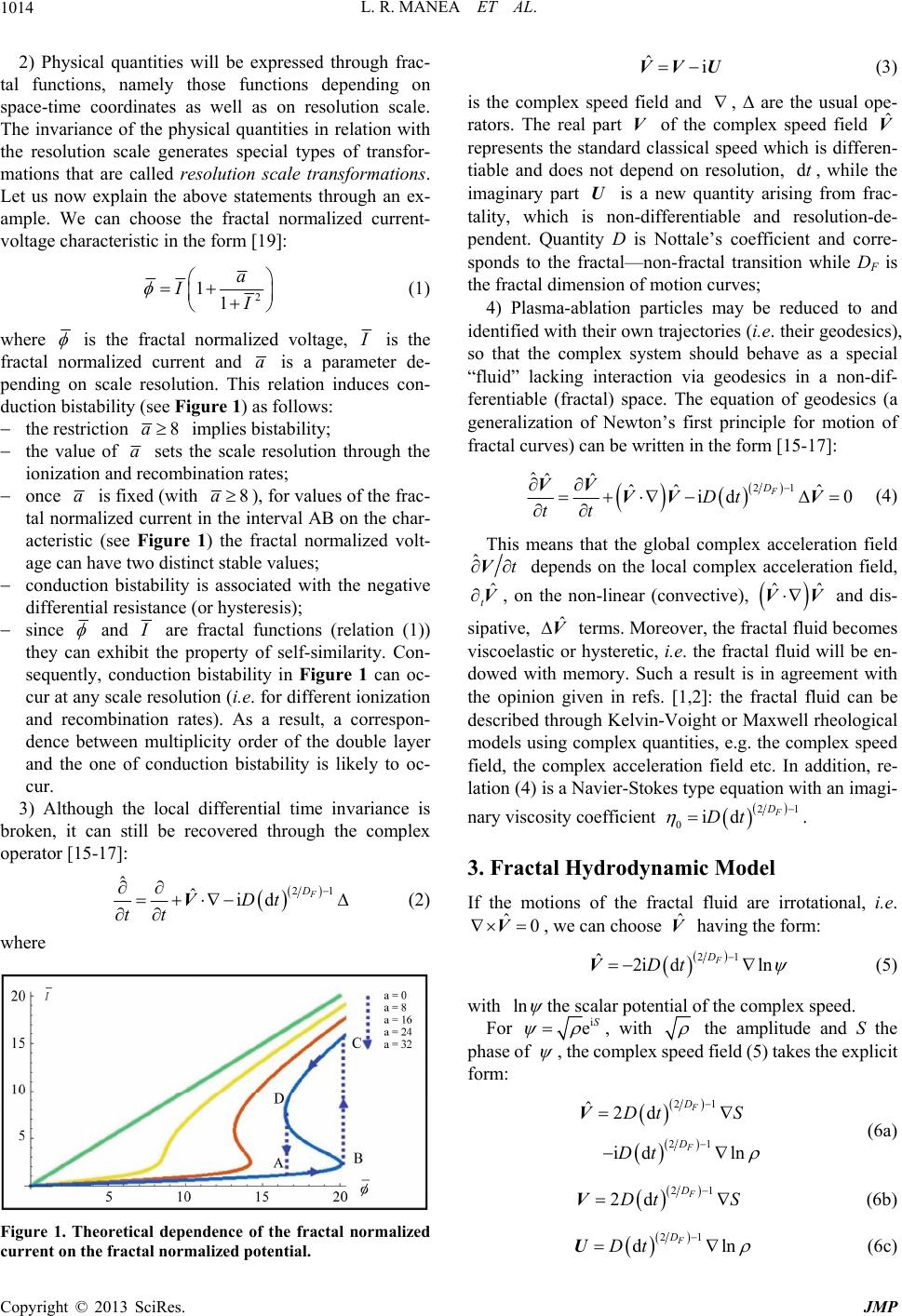 L. R. MANEA ET AL. 1014 ˆi VV U Vˆ V dt U 2) Physical quantities will be expressed through frac- tal functions, namely those functions depending on space-time coordinates as well as on resolution scale. The invariance of the physical quantities in relation with the resolution scale generates special types of transfor- mations that are called resolution scale transformations. Let us now explain the above statements through an ex- ample. We can choose the fractal normalized current- voltage characteristic in the form [19]: 2 11 a I (1) where is the fractal normalized voltage, I is the fractal normalized current and a is a parameter de- pending on scale resolution. This relation induces con- duction bistability (see Figure 1) as follows: the restriction 8a implies bistability; the value of a sets the scale resolution through the ionization and recombination rates; once a is fixed (with 8a), for values of the frac- tal normalized current in the interval AB on the char- acteristic (see Figure 1) the fractal normalized volt- age can have two distinct stable values; conduction bistability is associated with the negative differential resistance (or hysteresis); since and I are fractal functions (relation (1)) they can exhibit the property of self-similarity. Con- sequently, conduction bistability in Figure 1 can oc- cur at any scale resolution (i.e. for different ionization and recombination rates). As a result, a correspon- dence between multiplicity order of the double layer and the one of conduction bistability is likely to oc- cur. 3) Although the local differential time invariance is broken, it can still be recovered through the complex operator [15-17]: 21 id F D Dt ˆˆ tt V (2) where Figure 1. Theoretical dependence of the fractal normalized current on the fractal normalized potential. (3) is the complex speed field and , Δ are the usual ope- rators. The real part of the complex speed field represents the standard classical speed which is differen- tiable and does not depend on resolution, , while the imaginary part is a new quantity arising from frac- tality, which is non-differentiable and resolution-de- pendent. Quantity D is Nottale’s coefficient and corre- sponds to the fractal—non-fractal transition while DF is the fractal dimension of motion curves; 4) Plasma-ablation particles may be reduced to and identified with their own trajectories (i.e. their geodesics), so that the complex system should behave as a special “fluid” lacking interaction via geodesics in a non-dif- ferentiable (fractal) space. The equation of geodesics (a generalization of Newton’s first principle for motion of fractal curves) can be written in the form [15-17]: 21 ˆˆˆ ˆˆ ˆ id 0 F D Dt tt VV VVV (4) This means that the global complex acceleration field ˆt V ˆ t depends on the local complex acceleration field, V ˆˆ VV ˆ , on the non-linear (convective), and dis- sipative, V terms. Moreover, the fractal fluid becomes viscoelastic or hysteretic, i.e. the fractal fluid will be en- dowed with memory. Such a result is in agreement with the opinion given in refs. [1,2]: the fractal fluid can be described through Kelvin-Voight or Maxwell rheological models using complex quantities, e.g. the complex speed field, the complex acceleration field etc. In addition, re- lation (4) is a Navier-Stokes type equation with an imagi- nary viscosity coefficient 21 0id F D Dt ˆ0 . 3. Fractal Hydrodynamic Model If the motions of the fractal fluid are irrotational, i.e. Vˆ V , we can choose having the form: 21 ˆ2i dln F D Dt V ln (5) the scalar potential of the complex speed. with For i eS, with the amplitude and S the phase of , the complex speed field (5) takes the explicit form: 21 21 ˆ2d id ln F F D D DtS Dt V (6a) 21 2d F D Dt S V (6b) 21 dln F D Dt U (6c) Copyright © 2013 SciRes. JMP  L. R. MANEA ET AL. 1015 , y case in the form: Substituting (6a)-(6c) in (4) and separating the real and the imaginary parts up to an arbitrary phase factor which may be zero by a suitable choice of the phase of , we shall obtain: mQ VV 0 V t (7a) 0 V Q t (7b) with the fractal potential, 42 21 F D t U m 2D 2 0 2 0 0 2d d 2 F D QmDt mmD U (8) and 0 the rest mass of the fractal fluid particle. Equa- tion (7a) is the momentum conservation law, Equation (7b) is the density conservation law. They both define the fractal hydrodynamic model (FHM). Now, certain conclusions are evident: 1) Any particle is in permanent interaction with the “sub-fractal level” through the fractal potential Q; 2) The “sub-fractal level” is identified with a non- relativistic fractal fluid described by the probability den- sity and the momentum conservation laws—see relations ((7a), (7b)). These equations correspond to the general- ised quantum hydrodynamic model (GQHM). Indeed, for motions that can be described via fractal curves in fractal dimension F at Compton scale, 0 with the reduced Planck constant, the FHM reduces to a quantum hydrodynamic model (QHM). In this last case the “sub-fractal level” is identified with “sub-quantum level” [10-12]. 2Dm 3) The fractal potential (8) results from non-differen- tiability and should be considered as a kinetic term and not as a potential one. Moreover, the fractal potential (8) can generate a viscosity stress tensor type [15-17]. 42 2 0 ˆd , F D il il il li mD t UU xx il (9a) 21 dF D mDt ˆ iil l Q 0 1 2 (9b) whose divergence is equal to the usual force density as- sociated with Q (10) 4. Numerical Simulations Let us now rewrite the equations of FHM for the two- dimensional 2 xx xy VV VV tx yx (11a) 2 yxyy VVVV tx yy (11b) 0 xy VV tx y (11c) y y x eeV eV tx y V V exy (11d) e where fractal continuity equation of density energy was added [15-17]. With non-dimensional vario ables, ,t (12a) ,kx (12b) ,ky (12c) , x Vk V (12d) , y Vk V (12e) 0 ρN ρ (12f) in the case of the ideal gas and with variation σ being induced by the density and temperature variations , const.NT , Equations (11a)-(11d) be- comes: 2NT NVNVNV V (13a) 2NT NVNV VNV (13b) 0 NNV NV (13c) NT NTV NTV VV NT (13d) In Equations (13a)-(13d) the functional scaling rela- tion, 22 1k was considered. In a particular case, if we choose in (12a)-(12c) 0 corresponding to equilib- rium plasma density, ω to ion plasma frequency, and k to the inverse of Debye length, then α will be the square of the ion-acoustic speed and σ the kinetic pressure. Copyright © 2013 SciRes. JMP  L. R. MANEA ET AL. 1016 For numerical integration, the initial conditions, (14a) 0, ,0, (14b) 0, ,0,V V 10,,4 , (14c) N 10, ,4, (14d) 011 T anes, ,0,0, (14e) d the boundary on V (15a) ,1, 0, V (15b) ,0,0, V (15c) ,1, 0, V (15d) ,0,1 4, (15e) N ,1,1 4, (15f) N ,0,1 4, (15g) T ,1,14, (15h) ,,0 0, T V (15i) ,,1 0, V (15j) ,,0 0, ,,1 0, V (15k) V (15l) 22 22 14 12 expexp , 14 14 N 0 ,,0N (15m) ,,1 14,N (15n) 22 22 ,,0 14 12 expexp , 14 14 T T 0 (15o) ,,1 14.T (15p) are considered. In the boundary condition ((15m), (15o)) we assumed that the laser pulse which “hits” the target induces a plasma source that has a spatial-temporal Gaussian profile, similarly with the laser beam. N0 is the maximum normalized atom density, while T0 is the maximum normalized temperature which is assumed to be proportional with the laser beam energy, by preserv- ing the number of total released atoms. The equation system (13a)-(13d) with the initial con- di 2(a) ana)—τ llowing results are obtained: 1) the generation of ement with the experimental im tions (14a)-(14e) and the boundary ones (15a)-(15p) was numerically integrated via finite differences [20]. In Figures 2(a)-(c) space-dependence of the normalized density, N, normalized temperature, T, and in Figures 3(a)-(c) of the normalized velocities, Vξ and Vη, are given for the initial conditions, 00.4T, 01N and various normalized times: Figuresd 3( = 0.29, Fig- ures 2(b) and 3(b)—τ = 0.57, Figures 2(c) and 3(c)—τ = 0.88. The fo two plasma structures—see Figures 2(b), 3(b); 2) the symmetry of the normalized speed, Vξ, according to the axis symmetry of the space-time Gaussian; 3) shock waves and vertices at the plume periphery for the nor- malized speed field, Vη. These data are in agre ages at various evolution stages [5,6,21]. Moreover, if the current density of the particle is plotted on the sym- metry axis 12 —see Figures 4(a)-(c), for various distances frorget surface, a multi-peak structure as in [5,6] can be noticed. Increasing the value of the control parameter, , we conclude: 1) the arrival time of the first peak decreases; 2) the ratio between the first and the second maximum increases. This is in agreement with the experimental data according to which the parti- cles are gradually transferred from the fast into the slow part [22-24]; 3) the magnitude of the first maximum de- creases as a consequence of lateral expansion. There- fore we conclude that plume splitting is a hydrodynamic process similar to Gaussian disturbance emission. m the ta 5. Self-Similarity in Plasma Ablation (4) takes Neglecting the convection ˆˆ VV , Equation the form: 21 ˆˆ id F D Dt t VV=0 (16) or, separating the resolution scales, t 21 d0 F D Dt U (17) for the differentiable scale, and V 2 d0Dt 1 F D t V (18) for the fractal scale. Velocity fields are totally separated, U firstly applying Equations (17) and (18) to the Δ operator, i.e. 21 2 d0 F D Dt t VU (19) and 21 2 d0 F D Dt t UV (20) then, by substituting the dissipative terms via Equations Copyright © 2013 SciRes. JMP  L. R. MANEA ET AL. C JMP 1017 Figure 2. (a)-(c) Space-dependence of the normalized density, N, and normalized temperature, T, resulting from numerical 7) and (18), the Kirchhoff-type equations [25] result: simulations in Equations (13a)-(13d) for normalized initial conditions, T0 = 0.4, N0 = 1 and various normalized times: (a) τ = 0.29; (b) τ = 0.57; (c) τ = 0.88. opyright © 2013 SciRes. (1 i ;K,,1,2VU i (22d) take the unitary form [26]: 20 V 42 2 2d0 F D Dt t U (21) For the one-dimensional case, the previous equations w 42 42 ii 42 KK 0LT ith the substitutions: , L x (22a) , t T (22b) 442 2d, F D LDt (22c) 2 T onditions at (23) We impose “clamping” c1 for Equa- tion (23): 2 i K1, 20, (24a) 3 i 3 K1,0 (24b)  L. R. MANEA ET AL. 1018 Figure 3. (a)-(c) Space-dependence of normalized velocities, Vξ and Vη, resulting from numerical simulations of Equations (13a)-(13d) for normalized initial conditions, T0 = 0.4, N0 = 1 and various normalized times: (a) τ = 0.29; (b) τ = 0.57; (c) τ = 0.88. and for boundary conditions at 0 : ii0 K,0K, (26b) i K0, 0 (25) n i K0 , 0, These four boundary conditions i associated with the two initial ones i K,00 (26b) implies a unique solution i K, to Equation (23) Copyright © 2013 SciRes. JMP  L. R. MANEA ET AL. 1019 0. 0. 0. 0.8 1. 0.5 1. 1.5 (a) 0. 0. 0. 0.81. 0.2 0.4 0. 0. 1. j Figure 5. Numerical solution of the Kirchhoff Equation (23) with “clamped-free” unitary conditions, for a uniform ini- tial (b) 0. 0. 0. 0.8 1. 0. 0.4 0.6 0.8 1.0 (c) Figure 4. (a)-(c) Time-dependence of the particle current density on the symmetry axis (ξ = 1/2) resulting from nu- merical simulations for various normalized distances from the target surface: (a) = 0.19; (b) = 0.28; (c) = 0.42. —see Figure 5. Owig ng to scalin~ LtT, we find a solution for Equatio the form: n (23) in ii0 K, K i u (27) where the self-similarity variable is: , i0 i KK0 relaxes to zero within the first few time- steps. LtTx t (28) The boundary condition for u derives from i K conditions: 00, i u (29a) 00, i u (29b) 1 i u (29c) Substituting this self-similar form of i K, in Equation (23), the following equation for the self-similar solution i u results: 42 2 42 dd 43 dd ii uu d 0 i u d (30) The additional condition: 2 ( us ones, gives a unique self- similar solution to Equation (30): 2 d0 0, d i u 31) combined with the previo ii0 2K ,2K2π (32) see Figure 6, where the Fresnel sine integral, 2 sin π2d x Sxy y (33) een introduced. Relation (32) describes an oscillation via a self-similar solution 0 from the theory of diffraction has b t . This reflects the disp Equation (23). ersive nature of Copyright © 2013 SciRes. JMP 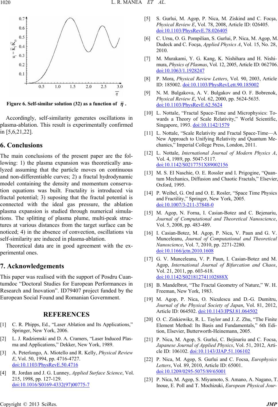 L. R. MANEA ET AL. 1020 Figure 6. Self-similar solution (n of 32) as a functio . Accordingly, self-similarity generates oscillations in plasma-ablation. This result is experimentally confirmed in [5,6,21,22]. 6. Conclusions The me z built. Fractality is introduced suposing that the fractal potential is e ideal gas pressure, the ablation ain conclusions of the present paper are thfol- wing: 1) the plasma expansion was theoretically ana- lo lyed assuming that the particle moves on continuous and non-differentiable curves; 2) a fractal hydrodynamic model containing the density and momentum conserva- tion equations was via fractal potential; 3) connected with th plasma expansion is studied through numerical simula- tions. The splitting of plasma plume, multi-peak struc- tures at various distances from the target surface can be noticed; 4) in the absence of convection, oscillations via self-similarity are induced in plasma-ablation. Theoretical data are in good agreement with the ex- perimental ones. 7. Acknowledgements This paper was realised with the support of Posdru Cuan- tumdoc “Doctoral Studies for European Performances in Research and Inovation”. ID79407 project funded by the European Social Found and Romanian Government. REFERENCES blation and Its Applications,” doi:10.1103/PhysRevE.50.4716 [1] C. R. Phipps, Ed., “Laser A Springer, New York, 2006. [2] L. J. Radziemski and D. A. Cramers, “Laser Induced Plas- ma and Applications,” Dekker, New York, 1989. [3] A. Peterlongo, A. Miotello and R. Kelly, Physical Re E, Vol. 50, 1994, pp. 4716-4727. view [4] R. Jordan and rface ScienceJ. G. Lunney, Applied Su, Vol. 215, 1998, pp. 127-129. doi:10.1016/S0169-4332(97)00775-7 [5] S. Gurlui, M. Agop, P. Nica, M. Ziskind and C. Focşa, Physical Review E, Vol. 78, 2008, Article ID: 026405. doi:10.1103/PhysRevE.78.026405 [6] C. Ursu, O. G. Pompilian, S. Gurlui Dudeck and C. Focşa, Applied Ph , P. Nica, M. Agop, M. ysics A, Vol. 15, No. 28, K. Nishihara and H. Nishi- , Article ID: 062706. 2010. [7] M. Murakami, Y. G. Kang, mura, Physics of Plasmas, Vol. 12, 2005 doi:10.1063/1.1928247 [8] P. Mora, Physical Review Letters, Vol. 90, 2003, Articl ID: 185002. e ett.90.185002doi:10.1103/PhysRevL 1103/PhysRevE.62.5624 [9] N. M. Bulgakova, A. V. Bulgakov and O. F. Bobrenok, Physical Review E, Vol. 62, 2000, pp. 5624-5635. doi:10. 1142/1579 [10] L. Nottale, “Fractal Space-Time and Microphysics: To- wards a Theory of Scale Relativity,” World Scientific, Singapore, 1993. doi:10. m Me- cs A, [11] L. Nottale, “Scale Relativity and Fractal Space-Time—A New Approach to Unifying Relativity and Quantu chanics,” Imperial College Press, London, 2011. [12] L. Nottale, International Journal of Modern Physi Vol. 4, 1989, pp. 5047-5117. doi:10.1142/S0217751X89002156 [13] M. S. El Naschie, O. E. Rossler and I. Prigogine, “Quan- tum Mechanics, Diffusion and Chaotic Fractals,” Elsevier, Oxford, 1995. [14] P. Weibel, G. Ord and O. E. Rosler, “Space Time Physics and Fractility,” Springer, New York, 2005. doi:10.1007/3-211-37848-0 [15] M. Agop, N. Forna, I. Casian Journal of Computational and The -Botez and C. Bejenariu, oretical Nanoscience, ournal of Computational and Theoretical Vol. 5, 2008, pp. 483-489. [16] I. Casian-Botez, M. Agop, P. Nica, V. Paun and G. V. Munceleanu, J Nanoscience, Vol. 7, 2010, pp. 2271-2280. doi:10.1166/jctn.2010.1608 [17] G. V. Munceleanu, V. P. Paun, I. Casian-Botez and M. Agop, International Journal of Bifurcation and Chaos, Vol. 21, 2011, pp. 603-618. doi:10.1142/S021812741102888X [18] B. Mandelbrot, “The Fractal Geometry of Nature,” W. H. Freeman, New York, 1983. [19] M. Agop, P. Nica, O. Niculescu and D.- Journal of the Physical Soci G. Dumitru, ety of Japan, Vol. 81, 2012, Article ID: 064502. doi:10.1143/JPSJ.81.064502 [20] O. C. Zinkiewikz, R. L. Taylor and J. Z. Zhu, “The Finite Element Method: Its Basis an tion, Elsevier, Butterworth-Heinema d Fundamentals,” 6th Edi- nn, 2005. Physics, Vol. 51, 2012, Arti- [21] P. Nica, M. Agop, S. Gurlui, C. Bejinariu and C. Focsa, Japanese Journal of Applied cle ID: 106102. doi:10.1143/JJAP.51.106102 [22] P. Nica, M. Agop, S. Gurlui and C. Focsa, Europhysics Letters, Vol. 89, 2010, Article ID: 65001. doi:10.1209/0295-5075/89/65001 [23] P. Nica, M. Agop, S. Miyamoto, S. Amano, A. Nagano, T. Inoue, E. Poll and T. Mochizuki, European Physical Jour- Copyright © 2013 SciRes. JMP  L. R. MANEA ET AL. Copyright © 2013 SciRes. JMP 1021 nal D, Vol. 60, 2010, pp. 317-323. doi:10.1140/epjd/e2010-00217-2 [24] P. Nica, S. Miyamoto, S. Amano, T. Inoue, A. Shimoura and T. Mochizuki, Physics Letters A, Vol. 370, 2007, pp. 154-157. doi:10.1016/j.physleta.2007.05.105 mbo, Z. Lu and I. To-[25] B. D. Coleman, E. H. Dill, M. Le bias, Archive for Rational Mechanics and Analysis, Vol. 121, 1993, pp. 339-359. doi:10.1007/BF00375625 [26] B. Audoly and S. Neukirch, Physical Review Letters, Vol. 95, 2005, Article ID: 095505. doi:10.1103/PhysRevLett.95.095505
|