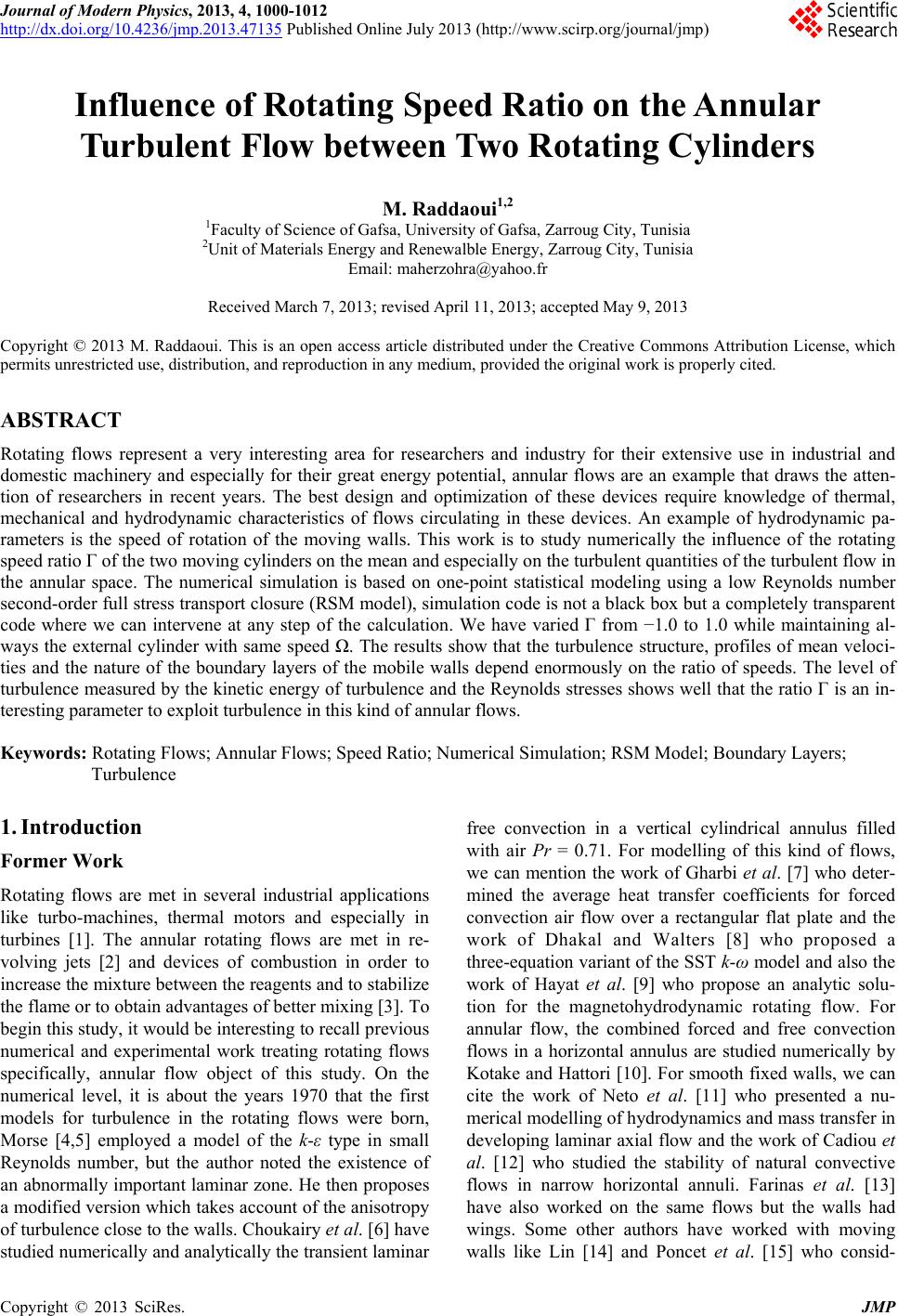
 Journal of Modern Physics, 2013, 4, 1000-1012 http://dx.doi.org/10.4236/jmp.2013.47135 Published Online July 2013 (http://www.scirp.org/journal/jmp) Influence of Rotating Speed Ratio on the Annular Turbulent Flow between Two Rotating Cylinders M. Raddaoui1,2 1Faculty of Science of Gafsa, University of Gafsa, Zarroug City, Tunisia 2Unit of Materials Energy and Renewalble Energy, Zarroug City, Tunisia Email: maherzohra@yahoo.fr Received March 7, 2013; revised April 11, 2013; accepted May 9, 2013 Copyright © 2013 M. Raddaoui. This is an open access article distributed under the Creative Commons Attribution License, which permits unrestricted use, distribution, and reproduction in any medium, provided the original work is properly cited. ABSTRACT Rotating flows represent a very interesting area for researchers and industry for their extensive use in industrial and domestic machinery and especially for their great energy potential, annular flows are an example that draws the atten- tion of researchers in recent years. The best design and optimization of these devices require knowledge of thermal, mechanical and hydrodynamic characteristics of flows circulating in these devices. An example of hydrodynamic pa- rameters is the speed of rotation of the moving walls. This work is to study numerically the influence of the rotating speed ratio of the two moving cylinders on the mean and especially on the turbulent quantities of the turbulent flow in the annular space. The numerical simulation is based on one-point statistical modeling using a low Reynolds number second-order full stress transport closure (RSM model), simulation code is not a black box but a completely transparent code where we can intervene at any step of the calculation. We have varied from 1.0 to 1.0 while maintaining al- ways the external cylinder with same speed . The results show that the turbulence structure, profiles of mean veloci- ties and the nature of the boundary layers of the mobile walls depend enormously on the ratio of speeds. The level of turbulence measured by the kinetic energy of turbulence and the Reynolds stresses shows well that the ratio is an in- teresting parameter to exploit turbulence in this kind of annular flows. Keywords: Rotating Flows; Annular Flows; Speed Ratio; Numerical Simulation; RSM Model; Boundary Layers; Turbulence 1. Introduction Former Work Rotating flows are met in several industrial applications like turbo-machines, thermal motors and especially in turbines [1]. The annular rotating flows are met in re- volving jets [2] and devices of combustion in order to increase the mixture between the reagents and to stabilize the flame or to obtain advantages of better mixing [3]. To begin this study, it would be interesting to recall previous numerical and experimental work treating rotating flows specifically, annular flow object of this study. On the numerical level, it is about the years 1970 that the first models for turbulence in the rotating flows were born, Morse [4,5] employed a model of the k-ε type in small Reynolds number, but the author noted the existence of an abnormally important laminar zone. He then proposes a modified version which takes account of the anisotropy of turbulence close to the walls. Choukairy et al. [6] have studied numerically and analytically the transient laminar free convection in a vertical cylindrical annulus filled with air Pr = 0.71. For modelling of this kind of flows, we can mention the work of Gharbi et al. [7] who deter- mined the average heat transfer coefficients for forced convection air flow over a rectangular flat plate and the work of Dhakal and Walters [8] who proposed a three-equation variant of the SST k-ω model and also the work of Hayat et al. [9] who propose an analytic solu- tion for the magnetohydrodynamic rotating flow. For annular flow, the combined forced and free convection flows in a horizontal annulus are studied numerically by Kotake and Hattori [10]. For smooth fixed walls, we can cite the work of Neto et al. [11] who presented a nu- merical modelling of hydrodynamics and mass transfer in developing laminar axial flow and the work of Cadiou et al. [12] who studied the stability of natural convective flows in narrow horizontal annuli. Farinas et al. [13] have also worked on the same flows but the walls had wings. Some other authors have worked with moving walls like Lin [14] and Poncet et al. [15] who consid- C opyright © 2013 SciRes. JMP 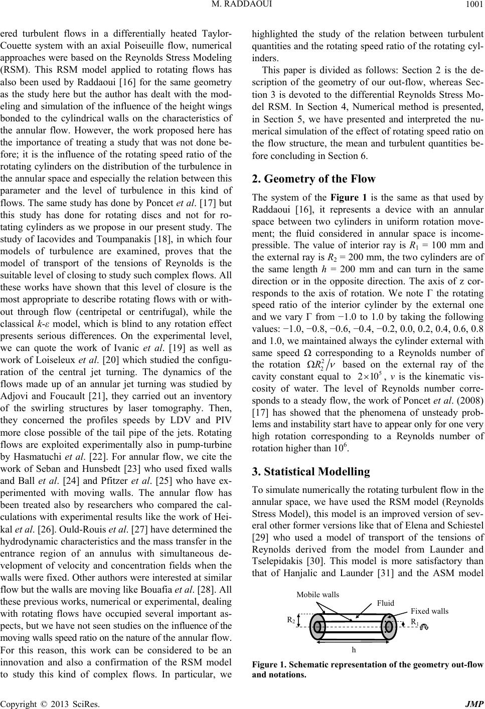 M. RADDAOUI 1001 ered turbulent flows in a differentially heated Taylor- Couette system with an axial Poiseuille flow, numerical approaches were based on the Reynolds Stress Modeling (RSM). This RSM model applied to rotating flows has also been used by Raddaoui [16] for the same geometry as the study here but the author has dealt with the mod- eling and simulation of the influence of the height wings bonded to the cylindrical walls on the characteristics of the annular flow. However, the work proposed here has the importance of treating a study that was not done be- fore; it is the influence of the rotating speed ratio of the rotating cylinders on the distribution of the turbulence in the annular space and especially the relation between this parameter and the level of turbulence in this kind of flows. The same study has done by Poncet et al. [17] but this study has done for rotating discs and not for ro- tating cylinders as we propose in our present study. The study of Iacovides and Toumpanakis [18], in which four models of turbulence are examined, proves that the model of transport of the tensions of Reynolds is the suitable level of closing to study such complex flows. All these works have shown that this level of closure is the most appropriate to describe rotating flows with or with- out through flow (centripetal or centrifugal), while the classical k-ε model, which is blind to any rotation effect presents serious differences. On the experimental level, we can quote the work of Ivanic et al. [19] as well as work of Loiseleux et al. [20] which studied the configu- ration of the central jet turning. The dynamics of the flows made up of an annular jet turning was studied by Adjovi and Foucault [21], they carried out an inventory of the swirling structures by laser tomography. Then, they concerned the profiles speeds by LDV and PIV more close possible of the tail pipe of the jets. Rotating flows are exploited experimentally also in pump-turbine by Hasmatuchi et al. [22]. For annular flow, we cite the work of Seban and Hunsbedt [23] who used fixed walls and Ball et al. [24] and Pfitzer et al. [25] who have ex- perimented with moving walls. The annular flow has been treated also by researchers who compared the cal- culations with experimental results like the work of Hei- kal et al. [26]. Ould-Rouis et al. [27] have determined the hydrodynamic characteristics and the mass transfer in the entrance region of an annulus with simultaneous de- velopment of velocity and concentration fields when the walls were fixed. Other authors were interested at similar flow but the walls are moving like Bouafia et al. [28]. All these previous works, numerical or experimental, dealing with rotating flows have occupied several important as- pects, but we have not seen studies on the influence of the moving walls speed ratio on the nature of the annular flow. For this reason, this work can be considered to be an innovation and also a confirmation of the RSM model to study this kind of complex flows. In particular, we highlighted the study of the relation between turbulent quantities and the rotating speed ratio of the rotating cyl- inders. This paper is divided as follows: Section 2 is the de- scription of the geometry of our out-flow, whereas Sec- tion 3 is devoted to the differential Reynolds Stress Mo- del RSM. In Section 4, Numerical method is presented, in Section 5, we have presented and interpreted the nu- merical simulation of the effect of rotating speed ratio on the flow structure, the mean and turbulent quantities be- fore concluding in Section 6. 2. Geometry of the Flow The system of the Figure 1 is the same as that used by Raddaoui [16], it represents a device with an annular space between two cylinders in uniform rotation move- ment; the fluid considered in annular space is income- pressible. The value of interior ray is R1 = 100 mm and the external ray is R2 = 200 mm, the two cylinders are of the same length h = 200 mm and can turn in the same direction or in the opposite direction. The axis of z cor- responds to the axis of rotation. We note the rotating speed ratio of the interior cylinder by the external one and we vary from 1.0 to 1.0 by taking the following values: 1.0, 0.8, 0.6, 0.4, 0.2, 0.0, 0.2, 0.4, 0.6, 0.8 and 1.0, we maintained always the cylinder external with same speed corresponding to a Reynolds number of the rotation 2 2 R based on the external ray of the cavity constant equal to , ν is the kinematic vis- cosity of water. The level of Reynolds number corre- sponds to a steady flow, the work of Poncet et al. (2008) [17] has showed that the phenomena of unsteady prob- lems and instability start have to appear only for one very high rotation corresponding to a Reynolds number of rotation higher than 106. 5 210 3. Statistical Modelling To simulate numerically the rotating turbulent flow in the annular space, we have used the RSM model (Reynolds Stress Model), this model is an improved version of sev- eral other former versions like that of Elena and Schiestel [29] who used a model of transport of the tensions of Reynolds derived from the model from Launder and Tselepidakis [30]. This model is more satisfactory than that of Hanjalic and Launder [31] and the ASM model Fixed walls R 2 Fluid Mobile walls R 1 h Figure 1. Schematic representation of the geometry out-flow and notations. Copyright © 2013 SciRes. JMP 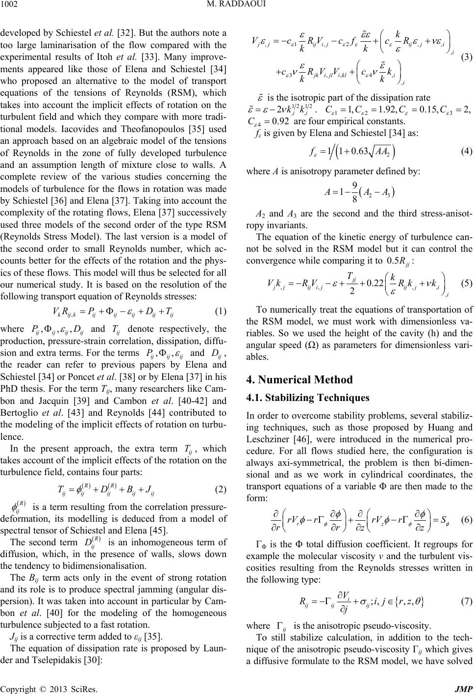 M. RADDAOUI 1002 developed by Schiestel et al. [32]. But the authors note a too large laminarisation of the flow compared with the experimental results of Itoh et al. [33]. Many improve- ments appeared like those of Elena and Schiestel [34] who proposed an alternative to the model of transport equations of the tensions of Reynolds (RSM), which takes into account the implicit effects of rotation on the turbulent field and which they compare with more tradi- tional models. Iacovides and Theofanopoulos [35] used an approach based on an algebraic model of the tensions of Reynolds in the zone of fully developed turbulence and an assumption length of mixture close to walls. A complete review of the various studies concerning the models of turbulence for the flows in rotation was made by Schiestel [36] and Elena [37]. Taking into account the complexity of the rotating flows, Elena [37] successively used three models of the second order of the type RSM (Reynolds Stress Model). The last version is a model of the second order to small Reynolds number, which ac- counts better for the effects of the rotation and the phys- ics of these flows. This model will thus be selected for all our numerical study. It is based on the resolution of the following transport equation of Reynolds stresses: ,1,2 ,, , 3,,4, , j jijijij ji i jkijli kli i k VcRVcfcR kk cRVV ck kk ,kij kijij VR Pijij ij D T ,PD (1) where ijij ijij ,, T ,P and ij denote respectively, the production, pressure-strain correlation, dissipation, diffu- sion and extra terms. For the terms ij , ij ij and ij , the reader can refer to previous papers by Elena and Schiestel [34] or Poncet et al. [38] or by Elena [37] in his PhD thesis. For the term Tij, many researchers like Cam- bon and Jacquin [39] and Cambon et al. [40-42] and Bertoglio et al. [43] and Reynolds [44] contributed to the modeling of the implicit effects of rotation on turbu- lence. D RR ijij ij BJ In the present approach, the extra term ij T, which takes account of the implicit effects of the rotation on the turbulence field, contains four parts: ij ij TD (2) ij is a term resulting from the correlation pressure- deformation, its modelling is deduced from a model of spectral tensor of Schiestel and Elena [45]. The second term ij is an inhomogeneous term of diffusion, which, in the presence of walls, slows down the tendency to bidimensionalisation. D The Bij term acts only in the event of strong rotation and its role is to produce spectral jamming (angular dis- persion). It was taken into account in particular by Cam- bon et al. [40] for the modeling of the homogeneous turbulence subjected to a fast rotation. Jij is a corrective term added to εij [35]. The equation of dissipation rate is proposed by Laun- der and Tselepidakis [30]: (3) is the isotropic part of the dissipation rate 12 12 2kk 3 1,1.92, 0.15,2,CCC C ,, ii . 12 0.92C 4 are four empirical constants. fε is given by Elena and Schiestel [34] as: 2 1 10.63AA (4) where A is anisotropy parameter defined by: 23 9 18 AA 0.5 A2 and A3 are the second and the third stress-anisot- ropy invariants. The equation of the kinetic energy of turbulence can- not be solved in the RSM model but it can control the convergence while comparing it to j R: ,, ,, , 0.22 2 jj j jijijij ji i Tk VkRVRk k (5) To numerically treat the equations of transportation of the RSM model, we must work with dimensionless va- riables. So we used the height of the cavity (h) and the angular speed () as parameters for dimensionless vari- ables. 4. Numerical Method 4.1. Stabilizing Techniques In order to overcome stability problems, several stabiliz- ing techniques, such as those proposed by Huang and Leschziner [46], were introduced in the numerical pro- cedure. For all flows studied here, the configuration is always axi-symmetrical, the problem is then bi-dimen- sional and as we work in cylindrical coordinates, the transport equations of a variable are then made to the form: rz rV rrV rS rrzz (6) is the total diffusion coefficient. It regroups for example the molecular viscosity ν and the turbulent vis- cosities resulting from the Reynolds stresses written in the following type: ;,, , i ij ijij V Rijrz j (7) where ij is the anisotropic pseudo-viscosity. To still stabilize calculation, in addition to the tech- nique of the anisotropic pseudo-viscosity ij which gives a diffusive formulate to the RSM model, we have solved Copyright © 2013 SciRes. JMP 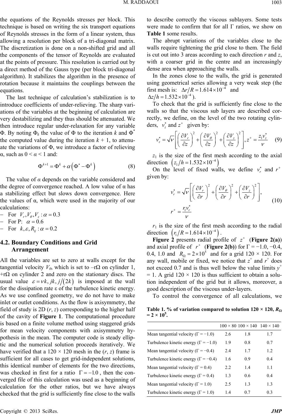 M. RADDAOUI 1003 the equations of the Reynolds stresses per block. This technique is based on writing the six transport equations of Reynolds stresses in the form of a linear system, thus allowing a resolution per block of a tri-diagonal matrix. The discretization is done on a non-shifted grid and all the components of the tensor of Reynolds are evaluated at the points of pressure. This resolution is carried out by a direct method of the Gauss type (per block tri-diagonal algorithm). It stabilizes the algorithm in the presence of rotation because it maintains the couplings between the equations. The last technique of calculation’s stabilization is to introduce coefficients of under-relieving. The sharp vari- ations of the variables at the beginning of calculation are very destabilizing and they thus should be attenuated. We then introduce regular under-relaxation for any variable . By noting k the value of to the iteration k and * the computed value during the iteration k + 1, to attenu- ate the variations of , we introduce a factor of relieving , such as 0 < α < 1 and: k ,,: 0V 1kk (8) The value of α depends on the variable considered and the degree of convergence reached. A low value of has a stabilizing effect but slows down convergence. Here the values of , which were used in the majority of our calculations: For .3 rz VV For P: 0.6 For .2 ij ,, :0kR 4.2. Boundary Conditions and Grid Arrangement All the variables are set to zero at walls except for the tangential velocity Vθ, which is set to –r on cylinder 1, +r on cylinder 2 and zero on the stationary discs. The usual value ,, 2kjkj k 1.0 is imposed at the wall for the dissipation rate of the turbulence kinetic energy. As we use confined geometry, we do not have to make inlet or outlet conditions. As the flow is axisymmetry, the field of study is 2D (r, z) corresponding to the higher half of the cavity of Figure 1. The computational procedure is based on a finite volume method using staggered grids for mean velocity components with axisymmetry hy- pothesis in the mean. The computer code is steady ellip- tic and the numerical solution proceeds iteratively. We have verified that a 120 × 120 mesh in the (r, z) frame is sufficient for all cases to get grid-independent solutions, this identical number of elements for the two directions, was checked in first for a ratio , then the con- verged file of this calculation was used as a beginning of calculation for the other ratios, but we have always checked that the grid is sufficiently fine close to the walls to describe correctly the viscous sublayers. Some tests were made to confirm that for all ratios, we show on Table 1 some results. The abrupt variations of the variables close to the walls require tightening the grid close to them. The field is cut out into 3 areas according to each direction r and z, with a coarser grid in the centre and an increasingly dense area when approaching the walls. In the zones close to the walls, the grid is generated using geometrical series allowing a very weak step (the first mesh is: 4 1.61410rR and 4 1.532 10zh and z vz ). To check that the grid is sufficiently fine close to the walls so that the viscous sub layers are described cor- rectly, we define, on the level of the two rotating cylin- ders, given by: 2 22 1 , rzz z V VVzv vz zzz (9) z1 is the size of the first mesh according to the axial direction 4 1.532 10zh and r vr 1 On the level of fixed walls, we define given by: 2 22 1 , rz r r V VV vrrr rv r (10) r1 is the size of the first mesh according to the radial direction 4 1.614 10rR z r 1 Figure 2 presents radial profile of (Figure 2(a)) and axial profile of . (Figure 2(b)) for = 1.0, 0.4, 0.4, 1.0 and and for a grid 120 × 120. For any wall, mobile or fixed, we notice that z+ and r+ does not exceed 0.7 and is thus well below the value limits y+ = 1. A grid 120 × 120 is thus sufficient to obtain a solu- tion independent of the grid but it allows, moreover, a good description of the viscous under-layers. 5 210R To control the convergence of all calculations, we Table 1. % of variation compared to solution 120 × 120, RΩ = 2 × 10⁵. 100 × 80 100 × 140140 × 140 Mean tangential velocity ( = 1.0) 2.6 1.8 1.7 Turbulence kinetic energy ( = 1.0) 1.9 0.8 0.7 Mean tangential velocity ( = 0.4) 2.4 1.7 1.2 Turbulence kinetic energy ( = 0.4) 1.6 0.9 0.4 Mean tangential velocity ( = 0.4) 2.2 1.4 1.1 Turbulence kinetic energy ( = 0.4) 1.3 0.6 0.4 Mean tangential velocity ( = 1.0) 2.5 1.3 1.3 Turbulence kinetic energy ( = 1.0) 1.4 0.7 0.3 Copyright © 2013 SciRes. JMP 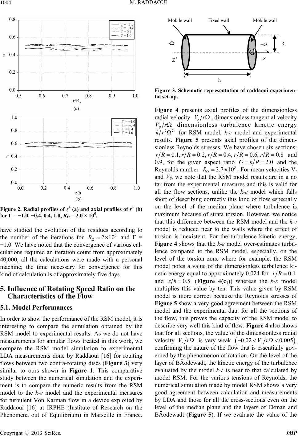 M. RADDAOUI 1004 Figure 2. Radial profiles of z+ (a) and axial profiles of r+ (b) for Γ = −1.0, −0.4, 0.4, 1.0, RΩ = 2.0 × 10⁵. have studied the evolution of the residues according to the number of the iterations for and = 1.0. We have noted that the convergence of various cal- culations required an iteration count from approximately 40,000, all the calculations were made with a personal machine; the time necessary for convergence for this kind of calculation is of approximately five days. 5 210R 5. Influence of Rotating Speed Ratio on the Characteristics of the Flow 5.1. Model Performances In order to show the performance of the RSM model, it is interesting to compare the simulation obtained by the RSM model to experimental results. As we do not have measurements for annular flows treated in this work, we compare the RSM model simulation to experimental LDA measurements done by Raddaoui [16] for rotating flows between two contra-rotating discs (Figure 3) very similar to ours shown in Figure 1. This comparative study between the numerical simulation and the experi- ment is to compare the numeric results from the RSM model to the k-ε model and the experimental measures for turbulent Von Karman flow in a device exploited by Raddaoui [16] at IRPHE (Institute of Research on the Phenomena out of Equilibrium) in Marseille in France. Z ’ Z + - h Mobile wall Fixed wall Mobile wall Figure 3. Schematic representation of raddaoui experimen- tal set-up. Figure 4 presents axial profiles of the dimensionless radial velocity r Vr , dimensionless tangential velocity Vr dimensionless turbulence kinetic energy 22 kr for RSM model, k-ε model and experimental results. Figure 5 presents axial profiles of the dimen- sionless Reynolds stresses. We have chosen six sections: 0.1, 0.2, 0.4, 0.6, 0.8rRrR rR rR rR and 0.9, for the given aspect ratio 2.0GhR 5 3.7 10R and the Reynolds number . For mean velocities Vr and Vθ, we note that the RSM model results are in a no far from the experimental measures and this is valid for all the flow sections, unlike the k-ε model which falls short of describing correctly this kind of flow especially on the level of the median plane where turbulence is maximum because of strata torsion. However, we notice that this difference between the RSM model and the k-ε model is reduced near to the walls where the effect of torsion is inexistent. For the turbulence kinetic energy, Figure 4 shows that the k-ε model over-estimates turbu- lence compared to the RSM model, especially, on the level of the torsion zone where for example, the RSM model notes a value of the dimensionless turbulence ki- netic energy equal to approximately 0.024 for 0.1rR and 0.5zh (Figure 4(c1)) whereas the k-ε model multiplies this value by ten. This value given by RSM model is more correct because the Reynolds stresses of Figure 5 show a very good agreement between the RSM model and the experimental data for all the sections of the flow, this proves the capacity of the RSM model to describe very well this kind of flow. Figure 4 also shows that for all sections, the value of the dimensionless radial velocity r Vr is very weak 0.02 0.005Vr r, confirming the nature of the flow that is essentially gov- erned by the phenomenon of rotation. On the level of the layer of BÄodewadt, the kinetic energy of the turbulence evaluated by the model k-ε is near to that calculated by model RSM. For the various tensions of Reynolds, the numerical simulation made by model RSM shows a very good agreement between calculation and measurements by LDA and those for all the cross-sections even on the level of the median plane and the layers of Ekman and BÄodewadt (Figure 5). If we evaluate the value of the Copyright © 2013 SciRes. JMP 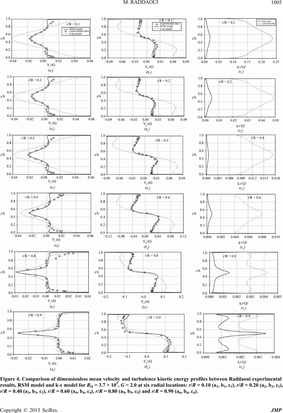 M. RADDAOUI Copyright © 2013 SciRes. JMP 1005 Figure 4. Comparison of dimensionless mean velocity and turbulence kinetic energy profiles between Raddaoui experimental results, RSM model and k-ε model for RΩ = 3.7 × 10⁵, G = 2.0 at six radial locations: r/R = 0.10 (a1, b1, c1), r/R = 0.20 (a2, b2, c2), r/R = 0.40 (a3, b3, c3), r/R = 0.60 (a4, b4, c4), r/R = 0.80 (a5, b5, c5) and r/R = 0.90 (a6, b6, c6). 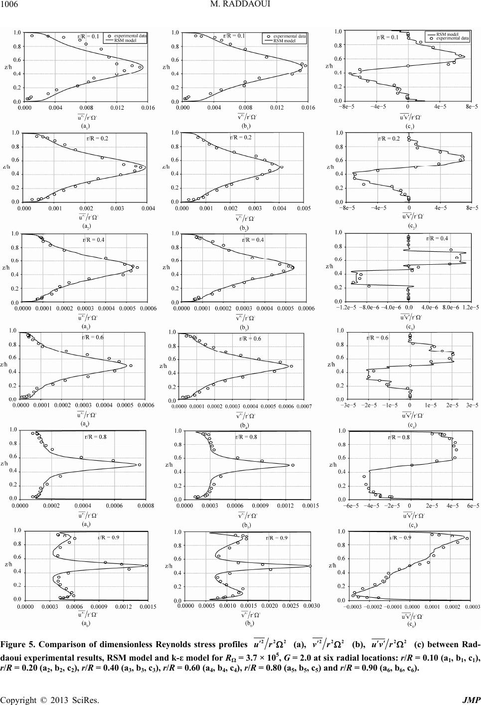 M. RADDAOUI 1006 Figure 5. Comparison of dimensionless Reynolds stress profiles ur 222 (a), vr 222 (b), uv r 22 (c) between Rad- daoui experimental results, RSM model and k-ε model for RΩ = 3.7 × 10⁵, G = 2.0 at six radial locations: r/R = 0.10 (a1, b1, c1), r/R = 0.20 (a2, b2, c2), r/R = 0.40 (a3, b3, c3), r/R = 0.60 (a4, b4, c4), r/R = 0.80 (a5, b5, c5) and r/R = 0.90 (a6, b6, c6). Copyright © 2013 SciRes. JMP  M. RADDAOUI Copyright © 2013 SciRes. JMP 1007 normal tensions of Reynolds 222 ur and 222 vr given by the model k- , we notice that 2 222 2222 23ur vrkr 0 1 0 5 210 5.3. Influence of the Rotating Speed Ratio on the Tangential Velocity For the mean quantities we chose to represent the radial variation tangential velocity on the median plane (Figure 7(a)) and the axial variation of this velocity in the centre of annular space (Figure 7(b)) for all values of the speed ratio specified previously because these regions are most significant for better observing the various phe- nomena especially those related to turbulence. The Rey- nolds number is always fixed equal to and the aspect ratio 1 the model k- over-estimates these tensions compared to model RSM. RSM model provides good results even in the boundary layers and models in a precise way the ten- sions of Reynolds. The behavior of the cross tensor is less well predicted in the layer of BÄodewadt. The second order model can now be used confidently to carry parametric studies even for different values of rotating speed ratio, as is the case in this study. We can then use this model to study the influence of rotating speed ratio on the structure, the level and the distribution of the turbulence of the flow in the annular space. GhR fixed at 2.0. For radial profile of tangential velocity (Figure 7(a)), we notice that there is not much effect if > 0, on the other hand for < 0 we note a little difference close to the interior cylinder. We can nevertheless note the following remarks: the boundary layer on the interior cylinder is crushed than that on the external cylinder and this is for all the ratios , we also notice that the profiles tangential velocity for 5.2. Influence of the Rotating Speed Ratio on the Structure of the Flow 1.0 and 1.0 don’t present a symmetry plane at the level of 2 All the cases studied correspond to a Reynolds number equal to 2.105 and the aspect ratio G = h/R1 fixed at 2.0. Figure 6 shows that the total structure of the flow de- pends enormously on the ratio number of revolutions , we notice that the swirls are more present if the two cyl- inders turn in the opposite direction with a parameter close to 1.0 (Figures 6(a) ( = 1.0), 6(b) ( = 0.8), 6(c) ( = 0.6), 6(d) ( = 0.4)), the swirls are definitely less present in the contrary case (Figures 6(a’) ( = 1.0), 6(b’) ( = 0.8), 6(c) ( = 0.6), 6(d’) ( = 0.4)) and to be completely absent for the very weak ratios (Figures 6(e) ( = 0.2), 6(f) ( = 0.0), 6(e’) ( = 0.2), 6(f’) ( = 0.0)). For the contra rotating cases , we notice the concentration of the maximum of swirls close to the interior cylinder, which is explained by the presence of a turbulence related to the phenomena of torsion but this turbulence is not maximum in the middle of annular space (for ), as we can think it, but rather near to the interior cylinder. More the number of revolutions of this cylinder decreases more these swirls disperse until disappearing completely for close to zero. We also notice that acts on the distribution of turbulence throughout the axis of the cylinders. Indeed, the swirls are more numerous on the level of the median plane for close to 1 and concentrates on the level of the fixed disks for a ratio close to 0.4. For the co rotating cases , turbulence is obviously much weaker, we notice that the swirls are distributed in a more uniform way on all the flow contrary to the contra rotating case. We also note that turbulence in this case is generated by gradient speed between the two cylinders than by the level of this speed. Finally we can also say that for the same ratio in absolute value, turbulence is more present at the level of the median plane in the co rotating case than in the contra rotating one. 0.75 rR as we can think it, because for these two cases, two cylinders turn with the same number of revo- lutions but the product r is not the same because the distance separating the cylinders from the axis of rotation is not the same one. For the axial evolution of tangential velocity (Figure 7(b)), we notice that the total form of these profiles depends enormously on the ratio . All these profiles are symmetrical compared to the median plane but the velocity is more uniform on all the space separating the two fixed disks for the ratio close to 0.4. For the values of close to 1.0, the profile of tan- gential velocity presents a maximum quit marked at the level of median plane. We notice also that the level of tangential velocity depends on the ratio, this level in- creases with this parameter: more this parameter increases more tangential velocity profiles is flattened, we can note also a presence of a central core for which is completely absent for other values of . 0.8 Concerning the tangential mean velocity we can say then that the ratio number of revolutions of the two cyl- inders is an important parameter for the study of the an- nular flows at the same time for the total structure of these flows and especially the nature of the boundary layers and the position of the maximum of this velocity in annular space. This kind of parameters appears very important then in the dimensioning and the optimization of certain machines utilizing the revolving flows in an annular space. 5.4. Influence of the Rotating Speed Ratio on the Turbulence Kinetic Energy The importance of this work appears especially by studying the influence of the speed ratio of rotation on the turbulent quantities, one as of these quantities is the tur- 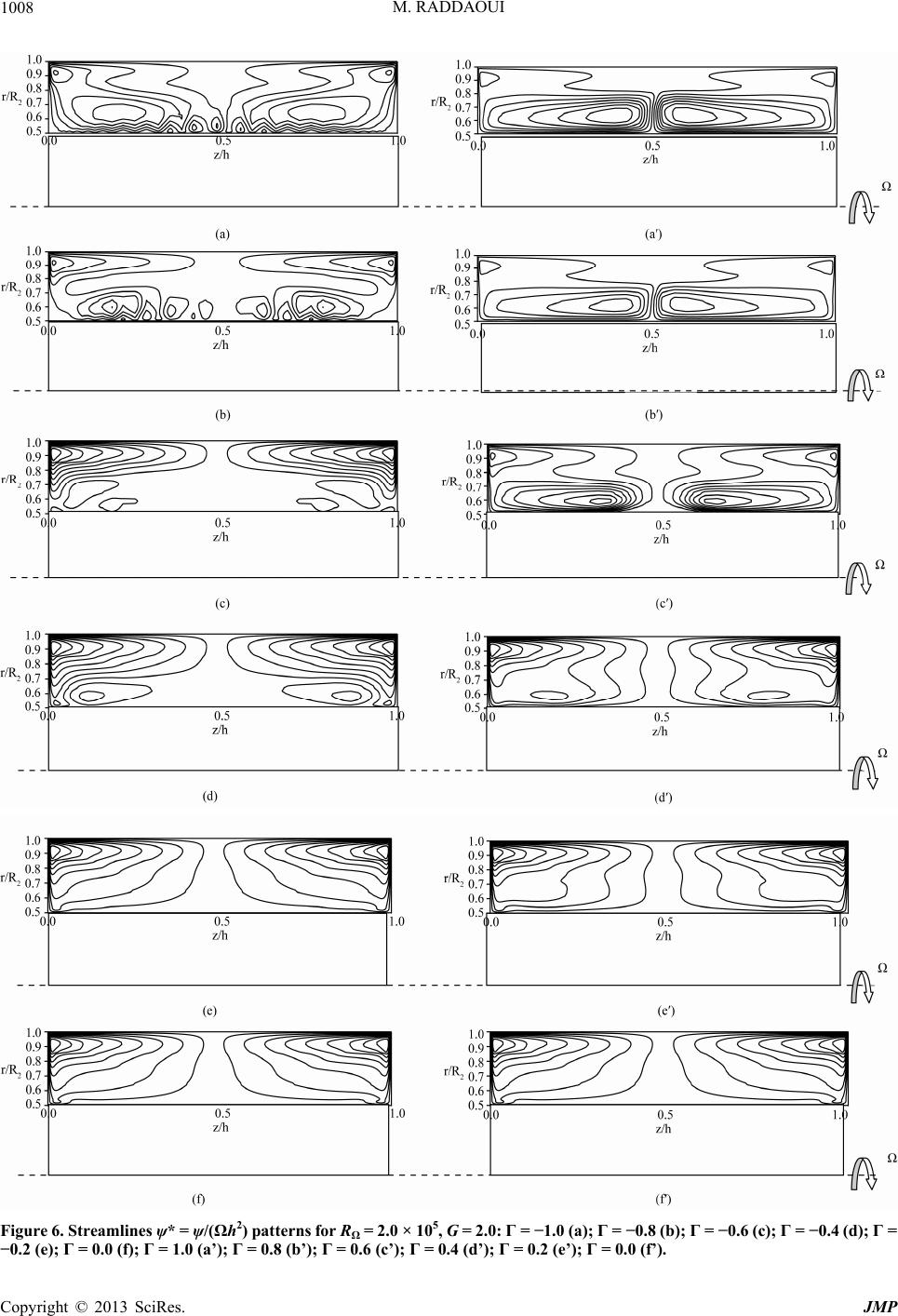 M. RADDAOUI 1008 Figure 6. Streamlines ψ* = ψ/(Ωh2) patterns for RΩ = 2.0 × 10⁵, G = 2.0: Γ = −1.0 (a); Γ = −0.8 (b); Γ = −0.6 (c); Γ = −0.4 (d); Γ = −0.2 (e); Γ = 0.0 (f); Γ = 1.0 (a’); Γ = 0.8 (b’); Γ = 0.6 (c’); Γ = 0.4 (d’); Γ = 0.2 (e’); Γ = 0.0 (f’). Copyright © 2013 SciRes. JMP 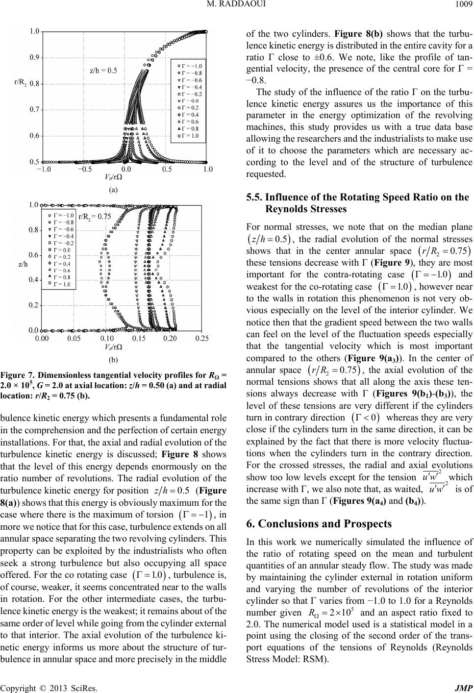 M. RADDAOUI 1009 of the two cylinders. Figure 8(b) shows that the turbu- lence kinetic energy is distributed in the entire cavity for a ratio close to ±0.6. We note, like the profile of tan- gential velocity, the presence of the central core for = 0.8. The study of the influence of the ratio on the turbu- lence kinetic energy assures us the importance of this parameter in the energy optimization of the revolving machines, this study provides us with a true data base allowing the researchers and the industrialists to make use of it to choose the parameters which are necessary ac- cording to the level and of the structure of turbulence requested. Vθ/r (a) 5.5. Influence of the Rotating Speed Ratio on the Reynolds Stresses For normal stresses, we note that on the median plane 0.5zh, the radial evolution of the normal stresses shows that in the center annular space 0.75rR 1.0 1.0 2 these tensions decrease with (Figure 9), they are most important for the contra-rotating case and weakest for the co-rotating case , however near to the walls in rotation this phenomenon is not very ob- vious especially on the level of the interior cylinder. We notice then that the gradient speed between the two walls can feel on the level of the fluctuation speeds especially that the tangential velocity which is most important compared to the others (Figure 9(a3)). In the center of annular space Vθ/r (b) 0.75rR 2, the axial evolution of the normal tensions shows that all along the axis these ten- sions always decrease with ( Figures 9(b1)-(b3)), the level of these tensions are very different if the cylinders turn in contrary direction Figure 7. Dimensionless tangential velocity profiles for RΩ = 2.0 × 10⁵, G = 2.0 at axial location: z/h = 0.50 (a) and at radial location: r/R2 = 0.75 (b). 0 whereas they are very close if the cylinders turn in the same direction, it can be explained by the fact that there is more velocity fluctua- tions when the cylinders turn in the contrary direction. For the crossed stresses, the radial and axial evolutions show too low levels except for the tension bulence kinetic energy which presents a fundamental role in the comprehension and the perfection of certain energy installations. For that, the axial and radial evolution of the turbulence kinetic energy is discussed; Figure 8 shows that the level of this energy depends enormously on the ratio number of revolutions. The radial evolution of the turbulence kinetic energy for position 2 uw which increase with , we also note that, as waited, 2 uw 5 210R is of the same sign than (Figures 9(a4) and (b4)). 0.5zh 1 (Figure 8(a)) shows that this energy is obviously maximum for the case where there is the maximum of torsion , in more we notice that for this case, turbulence extends on all annular space separating the two revolving cylinders. This property can be exploited by the industrialists who often seek a strong turbulence but also occupying all space offered. For the co rotating case , turbulence is, of course, weaker, it seems concentrated near to the walls in rotation. For the other intermediate cases, the turbu- lence kinetic energy is the weakest; it remains about of the same order of level while going from the cylinder external to that interior. The axial evolution of the turbulence ki- netic energy informs us more about the structure of tur- bulence in annular space and more precisely in the middle 1.0 6. Conclusions and Prospects In this work we numerically simulated the influence of the ratio of rotating speed on the mean and turbulent quantities of an annular steady flow. The study was made by maintaining the cylinder external in rotation uniform and varying the number of revolutions of the interior cylinder so that varies from 1.0 to 1.0 for a Reynolds number given and an aspect ratio fixed to 2.0. The numerical model used is a statistical model in a point using the closing of the second order of the trans- port equations of the tensions of Reynolds (Reynolds Stress Model: RSM). Copyright © 2013 SciRes. JMP 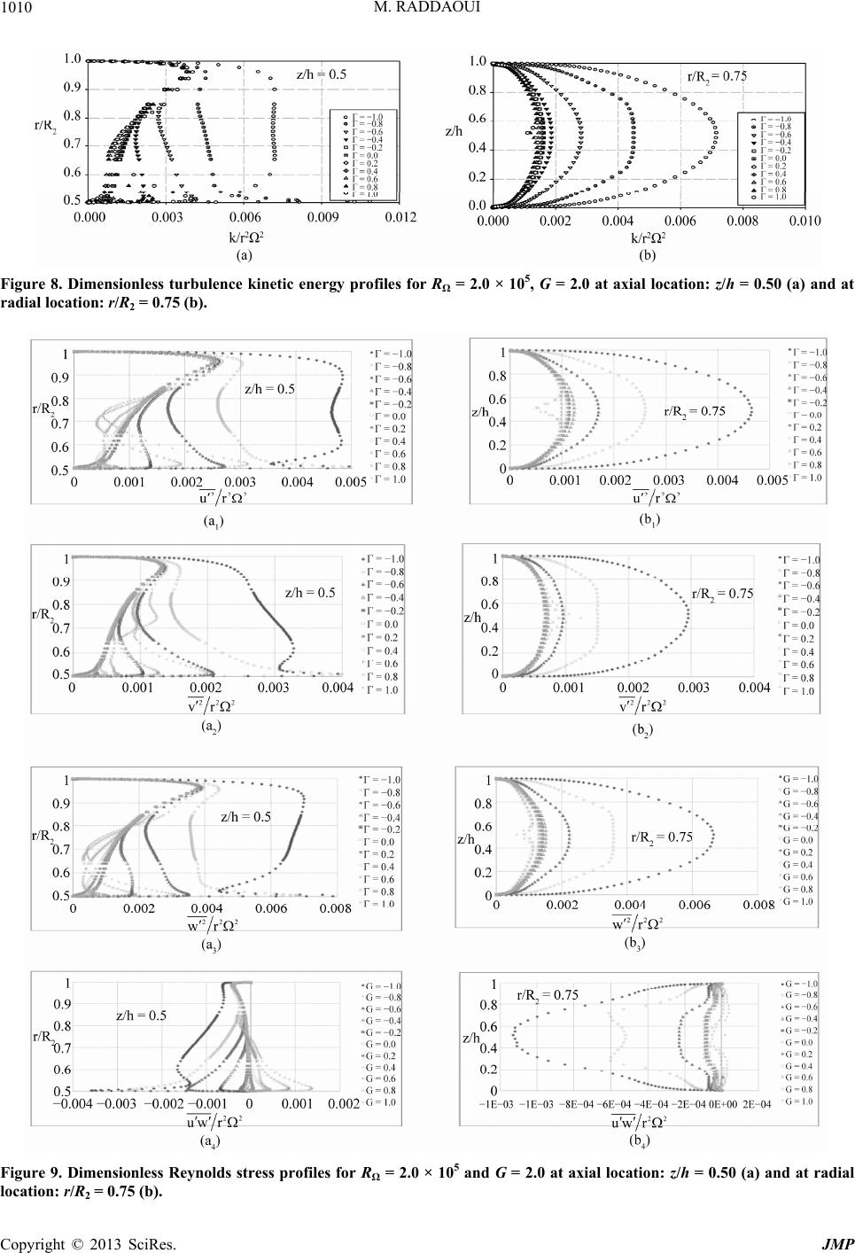 M. RADDAOUI 1010 Figure 8. Dimensionless turbulence kinetic energy profiles for RΩ = 2.0 × 10⁵, G = 2.0 at axial location: z/h = 0.50 (a) and at radial location: r/R2 = 0.75 (b). Figure 9. Dimensionless Reynolds stress profiles for RΩ = 2.0 × 10⁵ and G = 2.0 at axial location: z/h = 0.50 (a) and at radial location: r/R2 = 0.75 (b). Copyright © 2013 SciRes. JMP 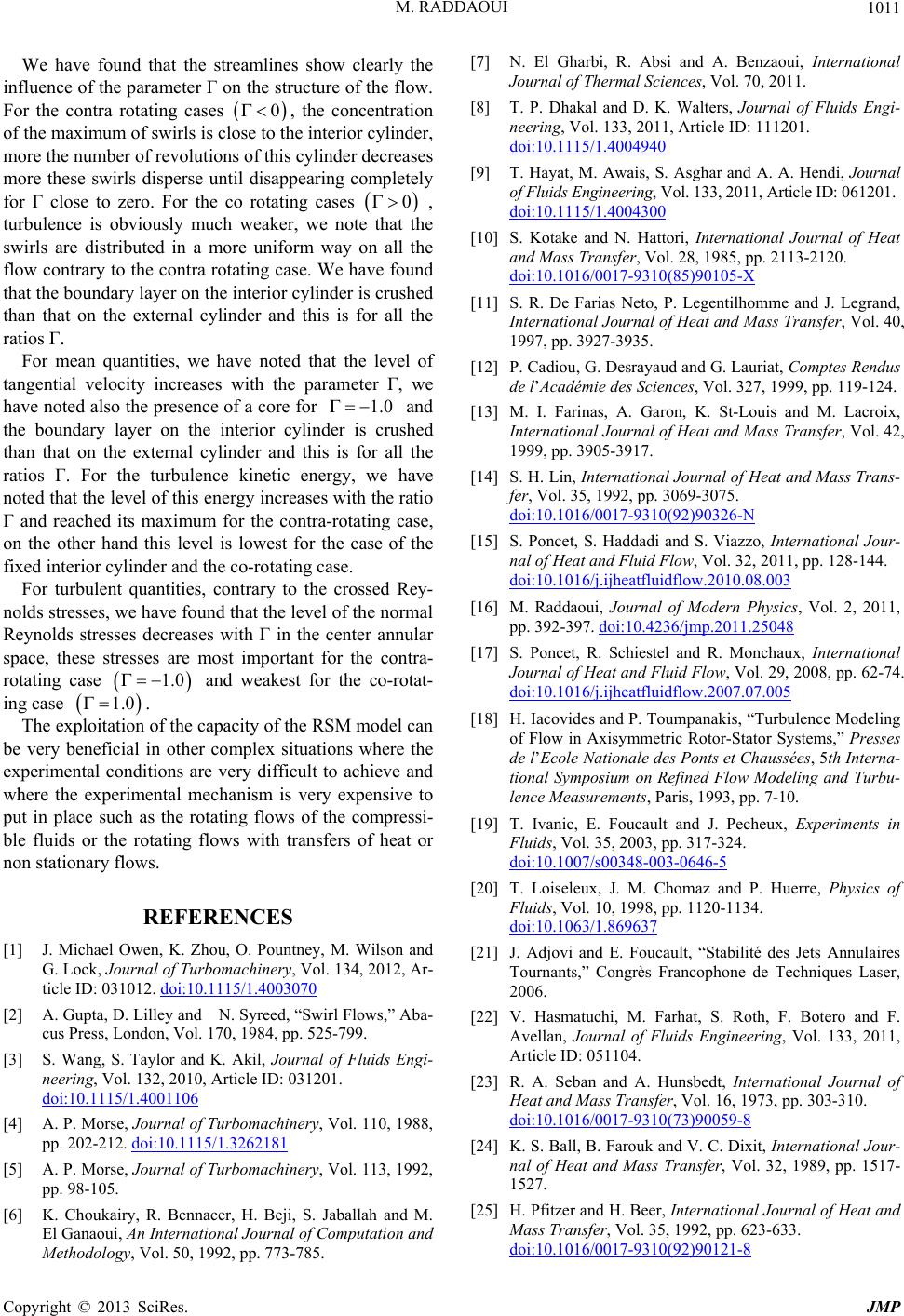 M. RADDAOUI 1011 We have found that the streamlines show clearly the influence of the parameter on the structure of the flow. For the contra rotating cases 0 , the concentration of the maximum of swirls is close to the interior cylinder, more the number of revolutions of this cylinder decreases more these swirls disperse until disappearing completely for close to zero. For the co rotating cases 0 , turbulence is obviously much weaker, we note that the swirls are distributed in a more uniform way on all the flow contrary to the contra rotating case. We have found that the boundary layer on the interior cylinder is crushed than that on the external cylinder and this is for all the ratios . For mean quantities, we have noted that the level of tangential velocity increases with the parameter , we have noted also the presence of a core for and the boundary layer on the interior cylinder is crushed than that on the external cylinder and this is for all the ratios . For the turbulence kinetic energy, we have noted that the level of this energy increases with the ratio and reached its maximum for the contra-rotating case, on the other hand this level is lowest for the case of the fixed interior cylinder and the co-rotating case. 1.0 1.0 1.0 For turbulent quantities, contrary to the crossed Rey- nolds stresses, we have found that the level of the normal Reynolds stresses decreases with in the center annular space, these stresses are most important for the contra- rotating case and weakest for the co-rotat- ing case . The exploitation of the capacity of the RSM model can be very beneficial in other complex situations where the experimental conditions are very difficult to achieve and where the experimental mechanism is very expensive to put in place such as the rotating flows of the compressi- ble fluids or the rotating flows with transfers of heat or non stationary flows. REFERENCES [1] J. Michael Owen, K. Zhou, O. Pountney, M. Wilson and G. Lock, Journal of Turbomachinery, Vol. 134, 2012, Ar- ticle ID: 031012. doi:10.1115/1.4003070 [2] A. Gupta, D. Lilley and N. Syreed, “Swirl Flows,” Aba- cus Press, London, Vol. 170, 1984, pp. 525-799. [3] S. Wang, S. Taylor and K. Akil, Journal of Fluids Engi- neering, Vol. 132, 2010, Article ID: 031201. doi:10.1115/1.4001106 [4] A. P. Morse, Journal of Turbomachinery, Vol. 110, 1988, pp. 202-212. doi:10.1115/1.3262181 [5] A. P. Morse, Journal of Turbomachinery, Vol. 113, 1992, pp. 98-105. [6] K. Choukairy, R. Bennacer, H. Beji, S. Jaballah and M. El Ganaoui, An International Journal of Computation and Methodology, Vol. 50, 1992, pp. 773-785. [7] N. El Gharbi, R. Absi and A. Benzaoui, International Journal of Thermal Sciences, Vol. 70, 2011. [8] T. P. Dhakal and D. K. Walters, Journal of Fluids Engi- neering, Vol. 133, 2011, Article ID: 111201. doi:10.1115/1.4004940 [9] T. Hayat, M. Awais, S. Asghar and A. A. Hendi, Journal of Fluids Engineering, Vol. 133, 2011, Article ID: 061201. doi:10.1115/1.4004300 [10] S. Kotake and N. Hattori, International Journal of Heat and Mass Transfer, Vol. 28, 1985, pp. 2113-2120. doi:10.1016/0017-9310(85)90105-X [11] S. R. De Farias Neto, P. Legentilhomme and J. Legrand, International Journal of Heat and Mass Transfer, Vol. 40, 1997, pp. 3927-3935. [12] P. Cadiou, G. Desrayaud and G. Lauriat, Comptes Rendus de l’Académie des Sciences, Vol. 327, 1999, pp. 119-124. [13] M. I. Farinas, A. Garon, K. St-Louis and M. Lacroix, International Journal of Heat and Mass Transfer, Vol. 42, 1999, pp. 3905-3917. [14] S. H. Lin, International Journal of Heat and Mass Trans- fer, Vol. 35, 1992, pp. 3069-3075. doi:10.1016/0017-9310(92)90326-N [15] S. Poncet, S. Haddadi and S. Viazzo, International Jour- nal of Heat and Fluid Flow, Vol. 32, 2011, pp. 128-144. doi:10.1016/j.ijheatfluidflow.2010.08.003 [16] M. Raddaoui, Journal of Modern Physics, Vol. 2, 2011, pp. 392-397. doi:10.4236/jmp.2011.25048 [17] S. Poncet, R. Schiestel and R. Monchaux, International Journal of Heat and Fluid Flow, Vol. 29, 2008, pp. 62-74. doi:10.1016/j.ijheatfluidflow.2007.07.005 [18] H. Iacovides and P. Toumpanakis, “Turbulence Modeling of Flow in Axisymmetric Rotor-Stator Systems,” Presses de l’Ecole Nationale des Ponts et Chaussées, 5th Interna- tional Symposium on Refined Flow Modeling and Turbu- lence Measurements, Paris, 1993, pp. 7-10. [19] T. Ivanic, E. Foucault and J. Pecheux, Experiments in Fluids, Vol. 35, 2003, pp. 317-324. doi:10.1007/s00348-003-0646-5 [20] T. Loiseleux, J. M. Chomaz and P. Huerre, Physics of Fluids, Vol. 10, 1998, pp. 1120-1134. doi:10.1063/1.869637 [21] J. Adjovi and E. Foucault, “Stabilité des Jets Annulaires Tournants,” Congrès Francophone de Techniques Laser, 2006. [22] V. Hasmatuchi, M. Farhat, S. Roth, F. Botero and F. Avellan, Journal of Fluids Engineering, Vol. 133, 2011, Article ID: 051104. [23] R. A. Seban and A. Hunsbedt, International Journal of Heat and Mass Transfer, Vol. 16, 1973, pp. 303-310. doi:10.1016/0017-9310(73)90059-8 [24] K. S. Ball, B. Farouk and V. C. Dixit, International Jour- nal of Heat and Mass Transfer, Vol. 32, 1989, pp. 1517- 1527. [25] H. Pfitzer and H. Beer, International Journal of Heat and Mass Transfer, Vol. 35, 1992, pp. 623-633. doi:10.1016/0017-9310(92)90121-8 Copyright © 2013 SciRes. JMP  M. RADDAOUI 1012 [26] M. R. F. Heikal, P. J. Walklate and A. P. Hatton, Interna- tional Journal of Heat and Mass Transfer, Vol. 20, 1977, pp. 763-771. doi:10.1016/0017-9310(77)90174-0 [27] M. Ould-Rouis, A. Salem, J. Legrand and C. Nouar, In- ternational Journal of Heat and Mass Transfer, Vol. 38, 1995, pp. 953-967. doi:10.1016/0017-9310(94)00233-L [28] M. Bouafia, A. Ziouchi, Y. Bertin and J.-B. Saulnier, International Journal of Thermal Sciences, Vol. 38, 1999, pp. 547-559. doi:10.1016/S0035-3159(99)80035-X [29] L. Elena and R. Schiestel, AIAA Journal, Vol. 33, 1995, pp. 812-821. doi:10.2514/3.12800 [30] B. E. Launder and D. P. Tselepidakis, International Jour- nal of Heat and Fluid Flow, Vol. 15, 1994, pp. 2-10. [31] K. Hanjalic and B. E. Launder, Journal of Fluid Mechan- ics, Vol. 74, 1976, pp. 593-610. doi:10.1017/S0022112076001961 [32] R. Schiestel, L. Elena and T. Rezoug, Numerical Heat Transfer, Vol. 24, 1993, pp. 45-65. [33] M. Itoh, Y. Yamada, S. Imao and M. Gonda, “Experi- ments on Turbulent Flow Due to an Enclosed Rotating Disc,” Proceedings of the International Symposium on Engineering Turbulence Modeling and Experiments, W. Rodi and E. N. Galic, Eds., Elsevier, New York, 1990, pp. 659-668. [34] L. Elena and R. Schiestel, International Journal of Heat and Fluid Flow, Vol. 17, 1996, pp. 283-289. doi:10.1016/0142-727X(96)00032-X [35] H. Iacovides and I. P. Theofanopoulos, International Jour- nal of Heat and Fluid Flow, Vol. 12, 1991, pp. 2-11. doi:10.1016/0142-727X(91)90002-D [36] R. Schiestel, “Les Ecoulements Turbulents,” 2nd Edition, Hermès, Paris, 1998. [37] L. Elena, “Modélisation de la Turbulence Inhomogène en Présence de Rotation,” Ph.D. Thesis, Université Aix-Mar- seille I-II, 1994. [38] S. Poncet, M. P. Chauve and R. Schiestel, Physics of Flu- ids, Vol. 17, 2005, Article ID: 075110. doi:10.1063/1.1964791 [39] C. Cambon and L. Jacquin, Journal of Fluid Mechanics, Vol. 202, 1989, pp. 295-317. doi:10.1017/S0022112089001199 [40] C. Cambon, L. Jacquin and J. L. Lubrano, Physics of Fluids, Vol. A4, 1992, pp. 812-824. [41] C. Cambon, R. Rubinstein and F. S. Godeferd, New Jour- nal of Physics, Vol. 6, 2004, pp. 73-102. doi:10.1088/1367-2630/6/1/073 [42] C. Cambon, C. Teissedre and D. Jeandel, Journal de Mécanique Théorique et Appliquée, Vol. 4, 1985, pp. 629- 657. [43] J. P. Bertoglio, G. Charnay and J. Mathieu, Journal de Mécanique Théorique et Appliquée, Vol. 4, 1980, pp. 421- 443. [44] W. C. Reynolds, “Towards a Structure-Based Turbulence Model,” In: T. B. Gatski, S. Sarkar and C. G. Speziale, Eds., Studies in Turbulence, Springer-Verlag, Berlin, 1991. [45] R. Schiestel and L. Elena, Aerospace Science and Tech- nology, Vol. 7, 1997, pp. 441-451. doi:10.1016/S1270-9638(97)90006-7 [46] P. G. Huang and M. A. Leschziner, “Stabilization of Re- circulation Flow Computations Performed with Second Moments Closures and Third Order Discretization,” Cor- nell University, Ithaca, 1985. Nomenclatures u R: Radius of disk (m) h: Height of cylinder (m) : Rotating speed ratio G: Aspect ratio R: Rotational Reynolds number Vz: Mean axial velocity Vr: Mean radial velocity Vθ: Mean tangential velocity : Axial velocity fluctuation v: Tangential velocity fluctuation w : Radial velocity fluctuation P: Pressure p: Pressure fluctuation : Density of fluid (kg·m3) : Kinematic viscosity of fluid (m2·s1) : Rotating velocity of disks (rad·s1) Copyright © 2013 SciRes. JMP
|