Open Journal of Applied Sciences, 2013, 3, 44-48
doi:10.4236/ojapps.2013.31B1009 Published Online April 2013 (http://www.scirp.org/journal/ojapps)
Imputed Empirical Likelihood for Varying Coefficient
Models with Missing Covariates
Peixin Zhao
Department of Mathematics, Hechi University, Guangxi Yizhou, China
Received 2013
ABSTRACT
The empirical likelihood-based inference for varying coefficient models with missing covariates is investigated. An
imputed empirical likelihood ratio function for the coefficient functions is proposed, and it is shown that iis limiting
distribution is standard chi-squared. Then the corresponding confidence intervals for the regression coefficients are
constructed. Some simulations show that the proposed procedure can attenuate the effect of the missing data, and
performs well for the finite sample.
Keywords: Empirical Likelihood; Varying Coefficient Model; Missing Covariate
1. Introduction
In practice, missing data frequ ently occur in many appli-
cation literatures, and the literatures on statistical analy-
sis of data with missing values have been flourished in
the past decade. Parametric regression models with miss-
ing data have been widely discussed (see [1,2]). In many
practical situations, however, the parametric regression
models are not flexible enough to capture the underlying
relation between the response and the associate covari-
ates. Hence, Wang [3] and Liang et al. [4] considered the
statistical inferences for the partially linear model with
missing covariates, which is a useful extension of the
parametric regression model. In addition, the following
varying coefficient model is another useful extension of
the parametric regression model, which has more imple-
ments and stronger explanations than the parametric re-
gression model. This paper aims to present an imputed
empirical likelihood method for analyzing the varying
coefficient model with covariate data missing at random.
Consider the following varying co efficient model

T
YX U

  (1)
where Y is the response variable, X is the covariate
vector, U is the scalar covariate, and 1p
  

1
uu  ,, T
pu
 
is a vector of unknown smooth functions. The error

has mean zero conditional on X and U. In this paper, we
focus mainly on the case that the covariate X may be
missing at random. That is, the available incomplete d ata
with the sample size of n are denoted as


,,,, 1,2,,
iiii
X
YU in  
where 0
i


if i
X
is missing, otherwise 1
i


, and
it satisfies that




1,, 1,
iiii iiii
PXYUPYUZ  ,  (2)
where


,
iii
Z
YU. The supposition (2) is commonly
used in the literature of missing data (see [2-5]). It is well
known that, in the presence of missing data, the complete
case analysis often generate a considerable bias and lose
efficiency. Then, it is important to develop some new
methods which can take the partially incomplete data
into account.
In this paper, an imputed empirical likelihood procedure
is proposed to study model (1) under missing covariates.
The proposed method can use the information of the in-
complete data efficiently, and the limiting distribution of
the proposed empirical log-likelihood ratio function is
shown to be standard chi-squared. Then the correspond-
ing confiden ce intervals of the regression coefficients are
constructed. Some simulations show that the proposed
procedure can attenuate the effect of missing data, and
performs well for finite sample.
Compared with the Wald-type confidence intervals,
the empirical likelihood based confidence intervals pos-
sess several attractive features such as the circumvention
of asymptotic variance estimation and the flexible shapes
of the confidence intervals determined by data (see [6]).
This paper provides an additional positive result of the
empirical likelihood inferences varying coefficient models
with missing data, which extends the application litera-
ture of the empirical likelihood method.
*This research was supported by the National Natural Science Founda-
tion of China (Grant No. 11101119).

P. X. ZHAO 45
2. Methodology and Main Results
Let
 
 
 
12
T
uiiii
i
zEXYX uZz
Yg zgzu


 
 ,
where
 
1
g
zEXZz and




2T
g
zEXXZz.
Then, by a simple calculation, we have that


 
1
0,
T ii
iiiiu ii
ii
EXYXU ZUufu







 




where i

i
Z
 , and

f
u is the density function
of i. Hence, using this information, an auxiliary ran-
dom vector can be defined as
U
  



1
,
T ii
iiii
i
hi
uXYXu Z
KU u

 





 




ui
i
where
 
h
K
uKuh, is a kernel function, and h
is the band w i d th. For a n y given u, note that

K
   
1,, n
uu   
are independent each other, and satisfy
 



0
i
Eu 

if and only if is the true parameter. Hence using
the empirical likelihood method proposed by [6], an em-

u 
pirical log-likelihood ratio function for can be defined
based on . However, contains the
unknown functions ,

u 
 
u 
 
iu

 
i

z 
1
g
z2 and

g
z, then it
can not be used directly for the statistical inference for
. A natural idea to solve this problem is to replace
,

u 

z 

1
g
z and

2
g
z with the following kernel
estimators respectively.









1
1
1
1
1
1
2
1
ˆ,
ˆ,
ˆ.
n
ih i
in
hi
i
n
ih i
in
hi
i
nT
ii hi
in
hi
i
KZ z
zKZ z
XK Zz
gz KZz
X
XK Zz
gz KZ z




















Then, we obtain the following estimated auxiliary ran-
dom vector
  



ˆ
ˆ1
ˆˆ
,
T
i
iiii
i
hi
uXYXu Z
KU u

 





 




i
ui
i

(3)
where


ˆˆ
ii
Z
  and 







12
ˆˆˆ
ui iii
Z
Yg ZgZu   .
Hence, an empirical log-likelihood ratio can be given by




  
111
ˆ
2maxlog0,1,1 .
nnn
iii ii
iii
Ru
np pppu





 




For any given u, provided that zero is inside the convex
hull of the points


  


1,, , n
u   u then a unique
value for




u
p
R  exists. By using the Lagrange mul-
tiplier method to find the optimal , then
i




Ru 
can be represented as
   

1
ˆ
2log1 ,
nTi
i
Ru u 




(4)
where

is a 1p

vector given as the solution to



  1
ˆ0.
ˆ
1
ni
T
ii
u
u

 



 (5)
Next we will show that is asymptotically chi-
square distributed when
 
Ru 



u 
R
is the true parameter for
given u. To derive a theory for , the following
assumptions will be required.
 
u 

Assumption 1. The bandwidth h satisfies that
and .
3
nh
 50nh 
Assumptio n 2. The k ernel function

K
u is a bounded
and symmetric probability density function, and satisfies


4
uKudu


.
Assumption 3. The density function


f
u is
bounded away from zero, and has continuous first de-
rivatives. The function


z  has bounded partial de-
rivatives up to the order 2 with .

inf 0
zz
 
Assumption 4.


u  ,


1
g
u and 2

g
u are twice
continuously differentiable. Furthermore, we assume that


0
ku



, 1, ,kp

, and

2
g
u is a positive defi-
nite matrix for any given u.
Assumption5. The error

and covariate X satisfy


4
supuEUu 

 and

4
supuEX U u

 ,
respectively, where

denotes the Euclidean distance.
Under these assumptions, the following theorem gives
the asymptotic distribution of .
 
Ru 
Theorem 1. Suppose that Assumptions 1-5 hold. For
any given u, if


u  is the true value of the parameter,
then




2,
D
p
Ru


where “D


2” denotes the convergence in distribution
and “
p

” denotes the chi-square distribution with p de-
grees of freedom.
By Theorem 1, the 1


confidence interval for


u 
can be defined as



 



,Cu uRu

 

where


satisfies


21
p
P




 . In addition, to

P. X. ZHAO
46
implement this estimation procedure, we need to choose
the bandwidth h. One can select h by optimizing some
data driven criteria, such as the classical criteria CV,
GCV and BIC. For the facilitation of calculation, we
suggest to choose the bandwidth based on the CV criteria.
More specifically, we can estimate h by minimizing the
following cross-validation score



2
[]
1
ˆ
CV ,
nT
iiiii
i
hYXU 



where is the estimator of after deleting
the ith subject. From our simulation experience, we
found that such a choice of the bandwidth is workable.

[]
ˆiu


u 
Next we give the proof Theorem 1. The proof the
Theorem 1 relies on the following lemma.
Lemma 1. Under the assumptions 1-5, we have
    
1
1ˆ0, ,
nD
i
i
uNvuu
nh




where and
 
2
vufuKsds
   


2
21
1,
Z
uE XEXZUu
ZZ








 



Proof. From the definition of in (3), it is
easy to show that
 
ˆiu







 
1
1
1
12
1ˆ
1
ˆ
1ˆ
1ˆ
n
i
i
nT
iiiih i
ii
niui hi
ii
u
nh
X
YX uKUu
nh
Z
KU u
nh
AA










 







(6)
Then, similar to the proof of Theorem 4 in Wang (2009),
we can prove that
 





11
21
11,
11
1.
niiihip
ii
niii ihi
ii
p
AXKUuo
Z
nh
A
EXZ K Uu
Z
nh
o
















Hence, using the central limit theorem, we have

 
1
0, ,
D

1
A
Nvu u (7)



2
0, ,
D

2
A
Nvu u (8)
where






2
vufuKsds,
  
2
11
uEX Uu
Z





 



and
 


2
2
1Z
uE EXZUu
Z




 


 





. Finally,
this lemma follows immediately by (6) - (8).
Proof of Theorem 1. Together with the proof of
Lemma 1 an d using the s ame argu ment as ar e used in the
proof of Lemma 1 in [7], we can show that
  

12
1ˆ
max .
ip
in uonh

 

(9)
Similar to the proof of (2.14) in [6], we can prove that


12 .
p
Onh 



(10)
Then, invoking (9) and (10), and applying the Taylor
expansion to (4), it is easy to show that




   


2
1
ˆˆ
22
nTT
ii
i
Ru
uu

  




1.
p
o 
(11)
Furthermore, from (5) and invoking (9) and (10), we
can prove that








1
11
12
ˆˆ ˆ
,
nn
T
ii i
ii
p
uu
onh
 








u
p
o
(12)
    
2
11
ˆˆ
1.
nn
TT
ii
ii
uu   




 (13)
Using (11)-(13), we obtain that
    
 
1
1
1
1ˆ
ˆ
1ˆ
.
T
n
i
i
n
i
i
Ruu u
nh
u
nh














(14)
where
    
1
1
ˆˆˆ
nT
ii
i
uu
nh
 



u. Invoking the
proof of the Lemma 1 and using the law of large numbers,
we obtain that


ˆ.
P
uvu

u
This together with (14) and Lemma 1 yields Theorem 1.
3. Simulation Studies
In this section, some Monte Carlo simulations are con-
ducted to evaluate the finite sample performance of the
proposed empirical likelihood method. The data are gen-
erated from the following model

,YXu




where




sin 2uu

 , the covariates U and X are
generated according to and

~0,1UU



~0,1XN ,

P. X. ZHAO 47
respectively. The response Y is generated according the
model with . In the following simulation
procedure, we choose the following two missing data
mechanism:

~0,0.5N 


Case1:

 
,
exp 10.50.450.5exp 10.50.45
yu
y
uy

 u
,
Case 2:


   
,
exp1 0.50.451exp1 0.50.45
yu
yu yu


The average missing rates of these two cases are 0.15
and 0.25 respectively. For each case, we take 1000 simu-
lation runs. In addition, the sample size is taken as n =
200.
For comparison, we consider two methods for construct-
ing the confiden ce intervals: the imputed estimation method
(IEL) proposed by this paper, and the naïve empirical
likelihood method (NEL). The latter is neglecting the
incomplete data information, and constructing the confi-
dence intervals for the regression coefficients only based
on the complete data. The averages of the confid ence in t er -
vals with the nominal level
1 95%,


 computed with
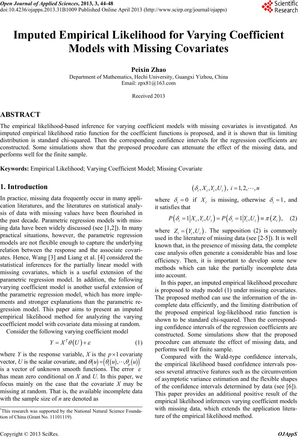
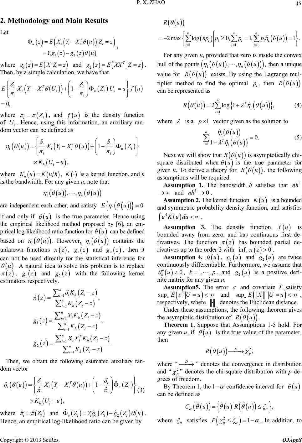
1000 simulation runs, are summarized in Figures 1 and 2.
Figure 1 is the simulation results under the missing
mechanism Case 1, and Figure 2 is the simulation results
under the missing mechanism Case 2, where the dashed
curves mean the results obtained by IEL method, the
dotted curves mean the results obtained by NEL method,
and the solid curve represents the real curve of


u  .
From Figures 1 and 2, we can make the following ob-
servations:
(i) The confidence intervals based on the I EL method
outperform those based on the NEL method, because
lengths of the confidence intervals obtained by the IEL
method are shorter than those obtained by the NEL method.
(ii) The performances of the confidence intervals based
on the IEL method are similar for all levels of missing
mechanisms. This implies that the imputed empirical
likelihood procedure can attenuate the effect of missing
Figure 1. The 95% confidence intervals of θ(u) under the
missing mechanism Case 1 based on IEL method (dashed
curve) and NEL method ( dotted curve).
Figure 2. The 95% confidence intervals of θ(u) under the
missing mechanism Case 2 based on IEL method (dashed
curve) and NEL method ( dotted curve).
data.
4. Conclusions and Discussions
We have proposed an imputed empirical likelihood pro-
cedure for varying coefficient models when some covari-
ates are missing. The proposed method can attenuate the
effect of missing data efficiently, and extends the impu-
tation-based estimation method to the varying coefficient
models with missing covariates. Simulation studies indi-
cated that the proposed method was very effective in at-
tenuating the effect of missing data and constructing the
confidence intervals for the coefficient functions.
In this paper, although we assume that all components
of the covariate are subject to missing, it is not essential.
The proposed estimation method can easily extend the
case that only some components of the covariate are
measured with missing. In addition, one useful extension
of the varying coefficient model is the varying coeffi-
cient partially linear model. For such model, Zhao and
Xue [8] considered the statistical inferences for regres-
sion coefficients when the response with missing. Then,
another interesting topic of further research is investigat-
ing the inferences for such varying coefficient partially
linear models with missing covariates.
REFERENCES
[1] Q. H. Wang and J. N. K. Rao, “Empirical Likelihood for
Linear Models under Imputation for Missing Responses,”
The Canadian Journal of Statistics, Vol. 29, No. 4，2001,
pp. 597-608 . doi：10.2307/3316009
[2] L. G. Xue, “Empirical Likelihood for Linear Models with
Missing Responses,” Journal of Multivariate Analysis,
Vol. 100, No. 7,2009, pp. 1353-1366.
doi：10.1016/j.jmva.2008.12.009
[3] Q. H. Wang, “Statistical Estimation in Partial Linear
Models with Covariate Data Missing at Random,” Annals
of the Institute of Statistical Mathematics, Vol. 61, No. 1,
2009, pp. 47-84.
doi:10.1007/s10463-007-0137-1
[4] H. Liang, S. J. Wang, J. M. Robbins and R. J. Carroll,
“Estimation in Partially Linear Models with Missing

P. X. ZHAO
48
Covariates,” Journal of the American Statistical
Association, Vol. 99, No. 466, 2004, pp. 357-367.
doi：10.1198/016214504000000421
[5] H. Wong, S. J. Guo, M. Chen and W.C. IP, “On Locally
Weighted Estimation and Hypothesis Testing of Varying
Coefficient Models with Missing Covariates,” Journal of
Statistical Planning and Inference, Vol. 139, No. 9, No. 1,
2009, pp. 2933-2951. doi：10.1016/j.jspi.2009.01.016
[6] A. B. Owen, “Empirical Likelihood Ratio Confidence
Regions,” The Annals of Statistics, Vol. 18, No. 1, 1990,
pp. 90-120. doi：10.1214/aos/1176347494
[7] L. G. Xue and L. X. Zhu, “Empirical Likelihood for a
Varying Coefficient Model with Longitudinal Data,”
Journal of the American Statistical Association, Vol. 102,
No. 478, 2007, pp. 642-654.
doi：10.1198/016214507000000293
[8] P. X. Zhao and L. G. Xue, “Variable Selection for
Semiparametric Varying Coefficient Partially Lin-
ear Models with Missing Response at Random,”
Acta Mathematica Sinica, English Series, Vol. 27,
No. 11, 2011, pp. 2 205-2216.
doi：10.1007/s10114-011-9200-1