 Journal of Modern Physics, 2013, 4, 66-77 doi:10.4236/jmp.2013.45B012 Published Online May 2013 (http://www.scirp.org/journal/jmp) Ground State of 4-7H Considering Internal Collective Rotation S. Paschalis1, G. S. Anagnostatos2* 1Lawrence Berkeley National Laboratory, Berkeley, California, 94720 USA 2Institute of Nuclear Physics, National Center for Scientific Research “Demokritos”, Aghia. Paraskevi, 15310 Greece Email: *anagnos4@otenet.gr Received 2013 ABSTRACT The g.s. of heavy and superheavy hydrogen isotopes, namely 4-7H, are successfully examined by applying the Isomor- phic Shell Model. Properties examined are binding energies and effective radii. The novelty of the present work is that, due to the small number of nucleons involved and the subsequently large deformation, an internal collective rotation appears which is inseparable from the usual internal motion even in the ground states of these nuclei, i.e., for such nu- clei the adiabatic approximation is not valid. This extra degree of freedom leads to a reduction of binding energies, an increase of effective radii, and an increase of level widths. Keywords: Hydrogen Isotopes 4H, 5H, 6H, and 7H; Cluster Models; Isomorphic Shell Model; Drip Lines; Internal Collective Rotation 1. Introduction Usage of secondary beams of short-lived radioactive nu- clei has enabled studies of nuclei near or beyond the lim- its of nuclear stability. During these studies very inter- esting new phenomena have been observed. In particular, the experimental study of heavy and superheavy hydro- gen isotopes is very interesting for several reasons: They are the closest to pure neutron nuclei and thus their study can provide information on neutron mat- ter. They are the simplest nuclear systems and their treatment could be relatively simple. They lie at the limit of nuclear stability (drip lines) and thus they may differ from ordinary nuclei. Even though they were the subject of many studies for over 40 years, their study is still incomplete. They exhibit an extreme fraction of neutron to proton ratio. They are the only nuclei with the 1s proton shell incomplete. They may provide information for testing and developing nuclear models. They may possess unusual structures, e.g., being very extended in space. They may provide knowledge for the physical meaning of a possible nuclear halo. They may provide a more precise definition of the limits of nuclear stability. Among the interesting references concerning hydrogen isotopes are [1-16]. Nevertheless, one has to admit that the experimental information and its interpretation available today are still contradictory and extremely lim- ited. Up to now, for the study of heavy and superheavy hy- drogen isotopes, several theoretical efforts were em- ployed, using different approaches. The present theoreti- cal treatment employs the same model, the Isomorphic Shell Model briefly summarized below in section 2, for all isotopes examined. This model employs the most probable forms and the average sizes of all nuclear shells which are attributed to two further utilized properties of nucleons, namely, their fermionic nature and their aver- age sizes. The first property alone is responsible for the most probable forms of nuclear shells and the second for their average sizes. Indeed: First, the anti-symmetric requirement of the wave function for nucleons results in a distribution for the maxima of this wave function which is equivalent to that obtained for the equilibrium of repulsive particles [17]. The repulsive property of nucleons is derived not only by this antisymmetrization, but also by the repulsive char- acter of the nuclear force itself being considered as originating due to the quark structure of the nucleons. The above equivalence replaces the nuclear many-body problem with that of finding the distribution of locations with maximum probability of repulsive particles on spheres *Corresponding author. Copyright © 2013 SciRes. JMP 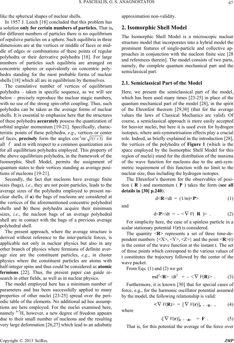 S. PASCHALIS, G. S. ANAGNOSTATOS 67 like the spherical shapes of nuclear shells. In 1957 J. Leech [18] concluded that this problem has a solution only for certain numbers of particles. That is, for different numbers of particles there is no equilibrium of repulsive particles on a sphere. Such equilibria in three dimensions are at the vertices or middle of faces or mid- dle of edges or combinations of these points of regular polyhedra or their derivative polyhedra [18]. For large numbers of particles such equilibria are arranged on concentric spheres or equivalently on concentric poly- hedra standing for the most probable forms of nuclear shells [18] which all are in equilibrium by themselves. The cumulative number of vertices of equilibrium polyhedra – taken in specific sequence, as we will see below – precisely reproduce the nuclear magic numbers, with no use of the strong spin-orbit coupling. Thus, such polyhedra can be taken as the average forms of nuclear shells. It is essential to emphasize here that the structures of these polyhedra accurately possess the quantization of orbital angular momentum [19-21]. Specifically, charac- teristic points of these polyhedra, e.g., vertices or center of faces, precisely form the angles cos-1m/ (1) for all and m with respect to a common quantization axis for all equilibrium polyhedra employed. This property of the above equilibrium polyhedra, in the framework of the Isomorphic Shell Model, permits the assignment of quantum states to their vertices standing as average posi- tions of nucleons [19-21]. Secondly, the fact that nucleons have average finite sizes (bags), i.e., they are not point particles, leads to the average sizes of the polyhedra employed to present nu- clear shells, if a) the bags of nucleons are considered at the vertices of the aforementioned concentric polyhedral shells and b) these polyhedra acquire their minimum sizes, i.e., the nucleon bags of an average polyhedral shell are in contact with the bags of a previous average polyhedral shell. The present approach, where the average structure is derived without reference to the inter-particle forces, is applicable not only in nuclear physics but also in any other branch of physics where fermions of definite aver- age size are the constituent particles, e.g., in cluster physics where the constituent particles are atoms with half-integer spins and thus could be considered as atomic fermions [22]. Thus, the present paper can guide re- search in other fields, as well as in nuclear physics. The model employed here has a minimum number of parameters and has been successfully applied to many properties of other nuclei [23-25] spread over the peri- odic table of the elements. No additional ad hoc assump- tions are here employed. For the nuclei examined here, namely 4-7H, however, a new degree of freedom appears due to their small number of nucleons and the resulting very large deformation [26,27] which lead to an adiabatic approximation non-validity. 2. Isomorphic Shell Model The Isomorphic Shell Model is a microscopic nuclear structure model that incorporates into a hybrid model the prominent features of single-particle and collective ap- proaches in conjunction with the nucleon finite size [28 and references therein]. The model consists of two parts, namely, the complete quantum mechanical part and the semiclassical part. 2.1. Semiclassical Part of the Model Here, we present the semiclassical part of the model, which has been used many times [23-25] in place of the quantum mechanical part of the model [28], in the spirit of the Ehrenfest theorem [29,30] (that for the average values the laws of Classical Mechanics are valid). Of course, a semiclassical approach is more easily accepted for heavier nuclei, but here it is used even for hydrogen isotopes, where anti-symmetrisation effects play a crucial role. Indeed, as briefly explained in the introduction [28], the vertices of the polyhedra of Figure 1 (which is the space employed by the Isomorphic Shell Model for this region of nuclei) stand for the distribution of the maxima of the wave function for nucleons due to the anti-sym- metric requirement of this function with no limit to the nuclear size, thus including the hydrogen isotopes. The Ehrenfest’s theorem for the observables of posi- tion ( R ) and momentum ( P ) takes the form (see all details in [30] p.240). d<R>/dt = (1/m)<P> (1) and d<P>/dt = - <V( R )> . (2) For simplicity here, the case of a spinless particle in a scalar stationary potential V(r) is considered. The quantity <R> represents a set of three time-de- pendent numbers {<X>, <Y>, <Z>} and the point <R>(t) is the center of the wave function at the instant t. The set of those points which correspond to the various values of t constitutes the trajectory followed by the center of the wave packet. From Eqs. (1) and (2) we get md2<R> /dt2 = - <V(R)> . (3) Furthermore, it is known [30] that for special cases of force, e.g., for the harmonic oscillator potential assumed by the model, the following relationship is valid: < V(R)> = [V(r)]r = <R> , (4) where -[ V(r)]r = <R> = F . (5) That is, for this potential the average of the force over Copyright © 2013 SciRes. JMP  S. PASCHALIS, G. S. ANAGNOSTATOS Copyright © 2013 SciRes. JMP 68 the whole wave function is rigorously equal to the clas- sical force F at the point where the center of the wave function is considered. Thus, for the special case of po- tential considered here, the motion of the center of the wave function precisely obeys the laws of classical me- chanics [30]. Any difference between the quantum and the classical description of the nucleon motion exclu- sively depends on the degree the wave function may be approximated by its center. Any such difference would contribute to deviations between the experimental data and the predictions of the semiclassical part of the model employed. Thus, in the present semiclassical treatment the nu- clear problem is reduced to that of studying the centers of the wave functions of the constituent nucleons or, in other words, of studying the average positions of these nucleons [26]. This is true without any restriction con- cerning the number of the constituent particles, i.e., if the nucleus is very light as here (hydrogen isotopes) or very heavy. We further proceed with the help of Figure 1 which is identical to that figure employed in [23-25], where the most probable forms and average sizes of the first three proton and the first three neutron shells are presented. It is essential to mention that these average sizes so lely depend on the average size of a proton, rp = 0.860 fm, and that of a neutron, rn = 0.974 fm. Each occupied ver- tex configuration of this figure corresponds to a quantum state configuration with definite angular momentum and energy. More details of the figure are given in its caption. The expressions of the two-body (two Yukawa) poten- tial V employed [31] for the present semi-classical treatment, of the kinetic energy T [32], of the spin-orbit energy VLS [33], of the intrinsic energy Eintr , of the rota- tional energy ER , and of the total binding energy EB are given in Eqs. (6) - (8) and (10) - (12), respectively. Iso- spin term in Eq.(10) is not needed since the isospin is here taken care of by the different shell structure (forms and sizes) between proton and neutron shells, as apparent from Figure 1. Vij= 0.993*1017*e-31.2334rij/rij-241.193* e-1.4546rij/rij (6) <T>nℓm = (ћ2/2M)[1/R 2max + ℓ (ℓ + 1)/ρ2nℓm] (7) ΣiVLiSi=λ Σi*( ћωi )2 /(h2/m)*ℓi si (λ = 0.03, the third parameter of the model (8) Figure 1. The space of the Isomorphic Shell Model for nuclei up to N = 20 and Z = 20. The equilibrium polyhedra in row 1 (2) stand for the most probable forms and average sizes of the first three neutron (proton). shells. The vertices of polyhedra (numbered as shown) stand for average positions of nucleons in definite quantum states (τ , n, ℓ, m, s). Central axes standing for the quantization of directions of the orbital angular momentum are labelled as nθℓ m and pass through the points marked by small solid circles. At the bottom-left of each block the numbering of this polyhedron proceeded by the letter Z (N) for protons (neutrons) is given. Over this the number of polyhedral vertices and the number of possible unoccupied vertices (holes, h) are also given. At the bottom-right of each block the radius of polyhedron is listed. Over this the cumulative num- ber of vertices of all previous polyhedra and of this polyhedron is also given. Finally, at the bottom-center of each block the distance ρnℓm of the nucleon average position nℓm from the relevant axis nθℓ m is given.  S. PASCHALIS, G. S. ANAGNOSTATOS 69 ћωi = (ћ2/M)(n+3/2)/<ri2> (9) Eintr.= ΣijVij - Σ<T>n m - ΣiVLiSi (10) ER = (ћ2/2M)I(I + 1) /2Θ (11) EB = Eintr - ER , (12) where • Vij is the potential energy between a pair of nucleons i, j at a distance rij, • n, ℓ, m are the quantum numbers characterizing a polyhedral vertex standing for the average position of a nucleon at the quantum state n, ℓ, m. • ℓi and s i stand for the orbital angular momentum quantum number ℓ and the intrinsic spin quantum num- ber s of any nucleon i. • M is the mass of a proton Mp or of a neutron Mn, • R max is the outermost proton or neutron polyhedral radius (R) plus the relevant average nucleon radius rp for a proton and rn for a neutron, (i.e., Rmax is the radius of the nuclear volume in which protons or neutrons are con- fined), • ρnℓm is the distance of a nucleon average position at a quantum state (n, ℓ, m from its orbital angular momen- tum at the direction nθ m , ) • I is the angular momentum of rotation (Here, of in- ternal collective rotation), and • Θ is the moment of inertia of collectively rotating nucleons. When only binding energies (and not scattering prop- erties) are required as here, just the second term of the above two-body potential of Eq.(6) would be sufficient. Thus, for non-scattering properties, the parameters of the model are the following five: the two-size parameters rp and rn, the two parameters from the second term of Eq.(6), and the one parameter, λ, from Eq.(8). With the help of these parameters all quantities Rmax, ρnℓm , ћωi, and Θ in Eqs.(6) - (12) are obtainable by employing the coordi- nates of the nucleon average positions given in the cap- tion of Figure 2. All these will become apparent in sec- tion 3 dealing with the applications on the different hy- drogen isotopes. Interesting applications of this version of the model on nuclear structure and reactions are included in Refs. [23- 25] and [34-35], respectively. In general, in order for the present results to have credibility concerning hydrogen isotopes and to show that these results do not depend on an ad hoc potential or on a set of adjustable parameters, we provide, beyond the applications on other nuclei, a rather detailed discussion concerning the potential and the parameters used in the model. 2.2. Two-Body Potential of the Model The potential of Eq. (6) is slightly stronger than that de- rived in [31]. This potential consists of one repulsive and another attractive Yukawa-type component, where each component involves two parameters describing its strength and range. The parameters of this potential were determined by examining its scattering and binding en- ergy properties. First, the potential was applied to the classical determination (using Newton’s equation for the two-body problem) of the first two moments [σ(1) (E) and σ(2)(E)] of the scattering of free nucleons at high energies. Second, the potential was applied to the semiclassical estimation of total binding energies of a set of even-even nuclei with N = Z in order for its saturation property to be checked for the correct nuclear size and, hence, nor- mal density. If just binding energy properties are required, as here, only the second term of Eq. (6) is sufficient. It is very interesting to comment on the fact that the potential employed here derived strictly from nuclear physics is very similar to that of N. Isgur [presented as an invited talk at the International Nuclear Physics confer- ence at Harrogate UK, V2 (1986) p.345] strictly derived from particle physics. Specifically, the central effective nucleon-nucleon potentials in the 3S1 and 1S0 channels arising from residual color forces (comprising the latest efforts to derive nuclear physics from the Quark Model with chromodynamics) are very similar to each other and to the potential of Eq. (6). Figure 2. Most probable forms and average sizes for the ground states of 4-7H. Numbering of spheres follows that of Figure 1. Neutrons (protons) are presented by light (dark) spheres. The central axes of internal collective rotations are shown as Ri.c.r. together with their coordinates. All distances dij between nucleons and ρij from the axes Ri.c.r. are determined from the coor- dinates x, y, z, i.e., (1): 0.974 cos450 , 0.974 cos450 , 0.000, (2): - 0.974 cos450 ,- 0.974 cos450 , 0.000, (5): 0.000, 2.511, 0.000, (6): 0.000, - 2.511, 0.000, (7): 2.511, 0.000, 0.000, (8): - 2.511, 0.000, 0.000., (3΄): 0.000, 0.000, 1.554. The quantum numbers τ, n, ℓ, m, s employed for the nucleon average positions in this figure are determined from Fig.1 via the angles nθℓ m and are (1): ½, 1, 0, 0, ½, (2): ½, 1, 0, 0, -1/2, (3) or (3’): -1/2, 1, 0, 0, ½, (5): ½, 1, 1, 1, ½, (6): ½, 1, 1, -1, -1/2, (7): ½, 1, 1, 1, -1/2, (8): ½, 1, 1, -1, ½, (9): ½, 1, 1, 0, ½, (10): ½, 1, 1, 0, -1/2. C opyright © 2013 SciRes. JMP 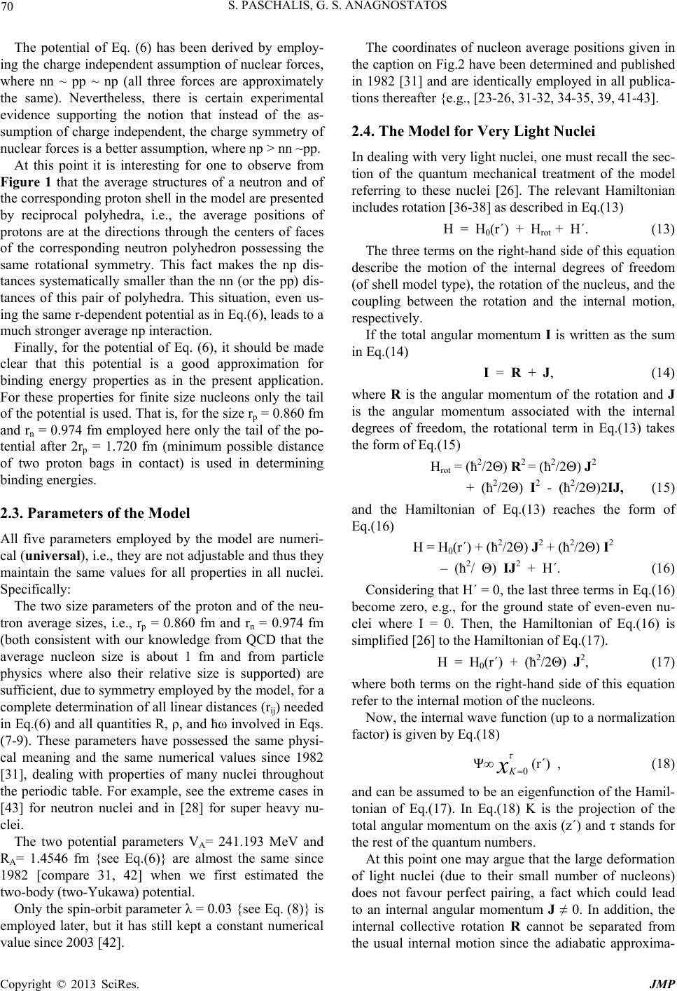 S. PASCHALIS, G. S. ANAGNOSTATOS 70 The potential of Eq. (6) has been derived by employ- ing the charge independent assumption of nuclear forces, where nn ~ pp ~ np (all three forces are approximately the same). Nevertheless, there is certain experimental evidence supporting the notion that instead of the as- sumption of charge independent, the charge symmetry of nuclear forces is a better assumption, where np > nn ~pp. At this point it is interesting for one to observe from Figure 1 that the average structures of a neutron and of the corresponding proton shell in the model are presented by reciprocal polyhedra, i.e., the average positions of protons are at the directions through the centers of faces of the corresponding neutron polyhedron possessing the same rotational symmetry. This fact makes the np dis- tances systematically smaller than the nn (or the pp) dis- tances of this pair of polyhedra. This situation, even us- ing the same r-dependent potential as in Eq.(6), leads to a much stronger average np interaction. Finally, for the potential of Eq. (6), it should be made clear that this potential is a good approximation for binding energy properties as in the present application. For these properties for finite size nucleons only the tail of the potential is used. That is, for the size rp = 0.860 fm and rn = 0.974 fm employed here only the tail of the po- tential after 2rp = 1.720 fm (minimum possible distance of two proton bags in contact) is used in determining binding energies. 2.3. Parameters of the Model All five parameters employed by the model are numeri- cal (universal), i.e., they are not adjustable and thus they maintain the same values for all properties in all nuclei. Specifically: The two size parameters of the proton and of the neu- tron average sizes, i.e., rp = 0.860 fm and rn = 0.974 fm (both consistent with our knowledge from QCD that the average nucleon size is about 1 fm and from particle physics where also their relative size is supported) are sufficient, due to symmetry employed by the model, for a complete determination of all linear distances (rij) needed in Eq.(6) and all quantities R, ρ, and ћω involved in Eqs. (7-9). These parameters have possessed the same physi- cal meaning and the same numerical values since 1982 [31], dealing with properties of many nuclei throughout the periodic table. For example, see the extreme cases in [43] for neutron nuclei and in [28] for super heavy nu- clei. The two potential parameters VA= 241.193 MeV and RA= 1.4546 fm {see Eq.(6)} are almost the same since 1982 [compare 31, 42] when we first estimated the two-body (two-Yukawa) potential. Only the spin-orbit parameter λ = 0.03 {see Eq. (8)} is employed later, but it has still kept a constant numerical value since 2003 [42]. The coordinates of nucleon average positions given in the caption on Fig.2 have been determined and published in 1982 [31] and are identically employed in all publica- tions thereafter {e.g., [23-26, 31-32, 34-35, 39, 41-43]. 2.4. The Model for Very Light Nuclei In dealing with very light nuclei, one must recall the sec- tion of the quantum mechanical treatment of the model referring to these nuclei [26]. The relevant Hamiltonian includes rotation [36-38] as described in Eq.(13) H = H0(r΄) + Hrot + H΄. (13) The three terms on the right-hand side of this equation describe the motion of the internal degrees of freedom (of shell model type), the rotation of the nucleus, and the coupling between the rotation and the internal motion, respectively. If the total angular momentum I is written as the sum in Eq.(14) I = R + J, (14) where R is the angular momentum of the rotation and J is the angular momentum associated with the internal degrees of freedom, the rotational term in Eq.(13) takes the form of Eq.(15) Hrot = (ћ2/2Θ) R2 = (ћ2/2Θ) J2 + (ћ2/2Θ) I2 - (ћ2/2Θ)2IJ, (15) and the Hamiltonian of Εq.(13) reaches the form of Eq.(16) H = H0(r΄) + (ћ2/2Θ) J2 + (ћ2/2Θ) I2 – (ћ2/ Θ) IJ2 + H΄. (16) Considering that H΄ = 0, the last three terms in Eq.(16) become zero, e.g., for the ground state of even-even nu- clei where I = 0. Then, the Hamiltonian of Eq.(16) is simplified [26] to the Hamiltonian of Eq.(17). H = H0(r΄) + (ћ2/2Θ) J2, (17) where both terms on the right-hand side of this equation refer to the internal motion of the nucleons. Now, the internal wave function (up to a normalization factor) is given by Eq.(18) Ψ∞ (r΄) , (18) xK 0 and can be assumed to be an eigenfunction of the Hamil- tonian of Eq.(17). In Eq.(18) K is the projection of the total angular momentum on the axis (z΄) and τ stands for the rest of the quantum numbers. At this point one may argue that the large deformation of light nuclei (due to their small number of nucleons) does not favour perfect pairing, a fact which could lead to an internal angular momentum J ≠ 0. In addition, the internal collective rotation R cannot be separated from the usual internal motion since the adiabatic approxima- C opyright © 2013 SciRes. JMP 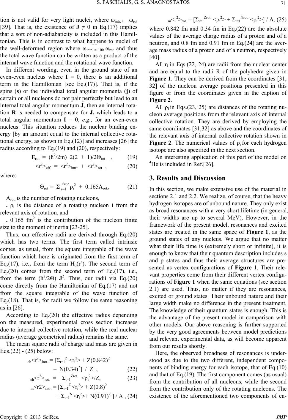 S. PASCHALIS, G. S. ANAGNOSTATOS 71 tion is not valid for very light nuclei, where ωintr. ≈ ωrot [39]. That is, the existence of J ≠ 0 in Eq.(17) implies that a sort of non-adiabaticity is included in this Hamil- tonian. This is in contrast to what happens to nuclei of the well-deformed region where ωintr. ≈ 100 ωrot and thus the total wave function can be written as a product of the internal wave function and the rotational wave function. In different wording, even in the ground state of an even-even nucleus where I = 0, there is an additional term in the Hamiltonian [see Eq.(17)]. That is, if the spins (s) or the individual total angular momenta (j) of certain or all nucleons do not pair perfectly but lead to an internal total angular momentum J, then an internal rota- tion R is needed to compensate for J, which leads to a total angular momentum I = 0, e.g., for an even-even nucleus. This situation reduces the nuclear binding en- ergy [by an amount equal to the internal collective rota- tional energy, as shown in Eq.(12)] and increases [26] the radius according to Eq.(19) and (20), respectively: Erot = (ћ2/2m) 2(2 + 1)/2Θrot , (19) <r2>eff. = <r2>intr. + <r2>rot , (20) where: Θrot =. Σ ρi2 + 0.165Arot., (21) Arot i1 Arot. is the number of rotating nucleons, . ρi is the distance of a rotating nucleon i from the relevant axis of rotation, and . 0.165 fm2 is the contribution of the nucleon finite size to the moment of inertia [23-25]. Thus, our effective radii are derived through Eq.(20) which has two terms. The first term called intrinsic comes, as usual, from the square integrable of the wave function which here is originated from the first term of Eq.(17), i.e., from the term H0(r΄). The second term of Eq.(20) comes from the second term of Eq.(17), i.e., from the term (ћ2/2Θ) J2. Thus, our radii via Eq.(20) come directly from the Hamiltonian of Eq.(17) and not from the square integrable of the wave function of Eq.(18). That is, for radii we follow the same reasoning as in [26]. According to Eq.(20) the effective radius depending on the measured, experimental cross section increases due to internal collective rotation, while the real nuclear radius (average geometrical radius) remains the same. The mean square radii of charge and mass are given in Eqs.(22) - (25) below: ch<r2>intr. = [Σι=1Ζ <ri2> + Z(0.842)2 – N(0.34)2] / Z , (22) ch<r2>rot. = Σι=1Ζrot. <ρi2>/Z, (23) m<r2>intr. = [Σι=1Ζ <ri2> + Z(0.8)2 + Σι=1N <ri2>+ N(0.91)2 ] / A , (24) m<r2>rot. = [Σι=1Ζrot. <ρi2> + Σι=1Nrot. <ρi2>] / A, (25) where 0.842 fm and 0.34 fm in Eq.(22) are the absolute values of the average charge radius of a proton and of a neutron, and 0.8 fm and 0.91 fm in Eq.(24) are the aver- age mass radius of a proton and of a neutron, respectively [40]. All ri in Eqs.(22, 24) are radii from the nuclear center and are equal to the radii R of the polyhedra given in Figure 1. They can be derived from the coordinates [31, 32] of the nucleon average positions presented in this figure or from the coordinates given in the caption of Figure 2. All ρi in Eqs.(23, 25) are distances of the rotating nu- cleon average positions from the relevant axis of internal collective rotation. They are derived by employing the same coordinates [31,32] as above and the coordinates of the relevant axis of internal collective rotation shown in Figure 2. The numerical values of ρi for each hydrogen isotope are also specified in the next section. An interesting application of this part of the model on 4He is included in Ref.[26]. 3. Results and Discussion In this section, we make extensive use of the material in sections 2.1 and 2.2. We realize, of course, that the heavy hydrogen isotopes are of unbound nature. They only exist as broad resonances with a very short lifetime (in general, their widths are up to several MeV). However, in the framework of the present model, resonances and excited states are treated in the same space of Figure 1, as the ground states of any nucleus. We argue that no matter what their life time is (extremely short or infinite), it is enough to know that their quantum description includes s and p states and thus their average structures are pre- sented as vertex configurations of Figure 1. Their rele- vant properties come from their different vertex configu- rations of Figure 1 when the same equations (see section 2.1) are used. Thus, no matter if they are resonances, excited or ground states. Their unbound nature and their large width make no difference in the present treatment. The knowledge of their quantum states is enough. This is the advantage of the present model in comparison with other models. Our above reasoning is further supported by the very good agreements between model predictions and relevant experimental data, as will become apparent from our results shortly. Here, the observed broadness of resonances is under- stood as due to the two different, independent compo- nents of binding energy for each isotope, that of Eq.(10) and that of Eq.(19). The first component comes (as usual) from the contribution of all nucleons, while the second from the contribution only of the rotating nucleons. The existence of the aforementioned two components of en- C opyright © 2013 SciRes. JMP  S. PASCHALIS, G. S. ANAGNOSTATOS 72 ergy is due to invalidity of the adiabatic approximation as earlier explained. Each of these two components has its own width around its own center and the observed broad width is their superimposition. As stated in the introduction, the space of the model, i.e., here that of Figure 1, is a necessary consequence of the anti-symmetrisation requirement of the total wave function for fermions (nucleons) and, as it should be, this space accurately possesses the quantization of orbital angular momentum [19-21]. Hence, Quantum Mechanics is inherent in the model space. Only the equations used (see section 2.1.1) are semiclassical. The same space of the model is employed for its purely quantum mechanical treatment [28]. This is a basic difference between the present semiclassical model and any other semiclassical treatment. In Figure 2 we provide the average g.s. structures ac- cording to the Isomorphic Shell Model for 4-7H, one iso- tope in each block of the figure. As apparent, these aver- age structures have cluster forms derived from Fig.1 by requiring maximum binding energy. All average neutron positions employed in this figure are identical to those of Figure 1 and are characterized with the same numbers. Two of the neutrons fill the two average positions in the neutron 1s shell (N1) numbered 1 and 2, while the va- lence neutrons 1 for 4H, 2 for 5H, 3 for 6H, and 4 for7H occupy average positions among the four equivalent av- erage positions in the neutron 1p shell (N2), numbered from 5 to 8. The 1s proton average position in Figure 1 numbered 3 is in the direction h – h of Z2 and pre-assumes that the proton shell Z2 is complete. How- ever, for the hydrogen isotopes examined here the proton average position numbered 3΄ is on the z axis as shown in all parts of Figure 2. This choice maximizes the dis- tances between the proton average position and the neu- tron average positions in 1p shell N2 as required by the antisymmetrization condition of the total wave function, which leads (as mentioned in the introduction [17]) to equivalent results with those of repulsive particles. In both Figures 1 and 2 the x axis passes through the points 7 and 8, while the y axis through the points 5 and 6. The quantization axis labelled q is defined by the average neutron positions 1 and 2, bisects the right angle of x, y axes [19-21], and passes through the middles of the edges 5, 7 and 11, 12, as shown in Figure 1 (see blocks N2 and Z2, respectively). Due to the very small number of particles, as seen from all parts of Figrue 2, the deformation is very large for the g.s. of all four isotopes examined. Thus, in these isotopes there are conditions for the internal angular momentum J which favour J ≠ 0 (section 2.2 ). Specifi- cally for each isotope: 4H. Here, we assume that the individual spins of each of the four nucleons of 4H couple to J = 2+, as internal angular momentum. This J ≠ 0 is responsible for the creation of an internal collective rotation R = 2+ to com- pensate for J, i.e., R = -J. The internal collective rotation R involves all four nucleons and the relevant axis of ro- tation is defined as follows. The valence neutron average position in the relevant block of Figure 2 is assigned to the position 8, however, it could be equivalently assigned to the average position 7 (both on x axis; see Figure 1), or even better it could be assigned in both positions with occupation probability 50% each. Then, the axis z is an axis of symmetry of the whole nucleus. Now, as usual, the axis of internal collec- tive rotation should be perpendicular to the axis of sym- metry and is taken in coincidence with the axis y. The relevant radii ρi for determining the moment of inertia via Eq.(21), according to Figure 2 and the rotating axis y, are: ρ3 = 1.554 fm, ρ1 = ρ2 = (0.974)cos450 ≈ 0.689 fm, and ρ8 = 2.511 fm. As seen from column 10 of Table1 the total moment of inertia is 10.33fm2 and this value is analysed in 2.58 fm2 for the proton and 7.75 fm2 for the three neutrons. 5H: Here, the individual spins of the four neutrons could couple to an internal angular momentum J = 2+, while the orbital angular momentum of the two 1p neu- trons (average positions 7 and 8 or equivalently 5 and 6) could couple to zero. Since J ≠ 0, an internal collective rotation R = 2+ is needed to compensate for J. This in- ternal collective rotation involves all five nucleon aver- age positions of 5H, i.e., the four responsible for the crea- tion of J = 2+ and one which follows the rotation (due to the average structure of the whole nucleus shown in Figure 2) of the previous four nucleon average positions. The axis of symmetry for the average structure of 5H shown in Figure 2 is again the axis z and now the axis of rotation could either be the y axis if the average positions of the two 1p neutrons are the 7 and 8, or equivalently, could be the x axis if the average positions of the two 1p neutrons are the 5 and 6. This double possibility results in an in-between axis as axis of rotation, that passing through the points 1 and 2, which is symbolised by xy and coincides with the quantization axis q. This axis, as should be, is perpendicular to the axis of symmetry z. The relevant radii ρi, for Eq.(21), according to Figure 2 and the rotating axis xy, are: ρ3 = 1.554 fm, ρ1 = ρ2 = 0, and ρ7 = ρ8 = (2.511)cos450 = 1.776 fm and as seen from column 10 of Table1 the total moment of inertia is 9.55 fm2 analysed in 2.58 fm2 for the proton and 6.97 fm2 for the four neutrons. 6H: Here, the two diametrically opposite neutrons in 3/2- state (average positions 7 and 8) could couple to J = 2+ {Figure 1k of Ref.[41]}. The internal collective rota- tion R = 2+ to compensate for J comes from only the average nucleon positions 7 and 8, which are responsible for this rotation. This axis of rotation is specified in C opyright © 2013 SciRes. JMP  S. PASCHALIS, G. S. ANAGNOSTATOS Copyright © 2013 SciRes. JMP 73 Ref.[41] (see Figure 1k) and passes through the origin and the point with coordinates 1, -1, 1. The relevant radii ρi for use in Eq.(21), according to Figure 2, are: ρ6 = ρ7 = 2.050 fm and the moment of inertia is 8.74 fm2 for the five neutrons. The proton does not participate in the in- ternal collective rotation and thus the rms charge radius does not increase due to this rotation. 7H. In this nucleus again two diametrically opposite neutrons (e.g., average positions 7 and 8), as discussed above, could couple to J = 2+, while the other two 3/2- neutrons (average positions 5 and 6) could couple to 0+. The internal collective rotation R and the relevant radii ρi are identical to those for 6H above. Again the proton does not participate in the internal collective rotation and thus does not increase the rms charge radius. In Table 1 the results obtained here are listed. Spe- cifically, in the col.1 of the table the four hydrogen iso- topes are listed, while in col.2 the numbers of the nu- cleon average positions of Figrue 1 occupied for each isotope are given by following Figure 2. In col.3 the total potential energy for each isotope is given by apply- ing Eq.(6) among all pairs of nucleons. In col.4 the cor- responding total energy due to spin orbit force is listed [Eqs.(8) and (9)], while in col.5 the total kinetic energy for each isotope is listed [Eq.(7)]. In col.6 the intrinsic energy is listed [Eq.(10)]. In col.12 the energy due to internal collective rotation is given [Eqs.(19, 21)] for the rotating nucleons listed in col.7 around the axis specified in col.8 and thus leading to the moment of inertia listed in col.9 of the table. In cols.13 and 14 the model binding energies in MeV [Eq.(12)] (4H/5.65, 5H/5.56, 6H/6.00, and 7H/7.68) and those of experiments [3, 7, 1, 15] (4H/~5.66, 5H/~5.48, 6H/5.38-6.18, and 7H/7.49-8.12) are shown, respectively. The very good agreements between these two groups of binding energies are apparent. In Table 1 we have employed binding energies instead of resonance energies which, of course, can be derived from the listed binding energies by subtracting the bind- ing energy of 3H equal to 8.48 MeV. For example for 4H the g.s. model binding energy from Table1 is 5.65 MeV, thus the resonance energy is 8.48 – 5.65 = 2.83 MeV which is in very good agreement with the predictio n 3.05 ± 0.19 of [13]. In cols.10 and 11 of Table 1 the effective, average ra- dii for charge and mass [Eqs.(22-23) and (24-25)], re- spectively, are listed. There are no experimental values for comparison. However, the large contribution to the relevant radii of the rotational component is apparent, particularly for the effective charge radii. Notice the great difference of the charge radii for 4H and 5H (i.e., 2.26 fm and 2.24 fm, respectively) in comparison to those of 6H and 7H (i.e., 1.57 fm and 1.54 fm, respec- tively), where for the first two nuclei the proton partici- pates in the internal collective rotation, while in the sec- ond two it does not. Finally, from Table 1 it is interesting for one to com- pare the intrinsic energies (col.6) with the rotational en- ergies (col.12). These two components of total binding energy (col. 13) for each hydrogen isotope are rather far apart. This remark supports the broad structure of g.s. resonances for 4-7H to be of the size of their total binding energies (cols. 13 and 14). The experimental widths are for 4H 5.14 ± 1.38 MeV [13], for 5H 5.4 ± 0.5 MeV [9], and for 6H 5.8 ± 2.0 MeV [16]. Up to now for 7H there are only indications for its production. Thus, there is not available an experimental value of width. The aforemen- tioned values of widths compare very well with our pre- dicted values 5.56, 5.45, and 5.85 MeV, respectively (col. 13 of Table 1). In addition, it is considered instructive to give below some more details concerning the calculations of the total kinetic energies in column five of Table 1 by applying Eq.(7) for each nucleon. The kinetic energy for the 1s proton is calculated ex- plicitly in Eq.(26) below. T1p in 1s state =( ћ2/2Mp)[(1-0.04)/(1.554+0.860)2 + 2(2+1)0.04/(1.5542+0.165)=5.349 MeV.(26) The first comment on this equation is that according to Ref.[42] for 3H, in order to obtain the experimental point proton momentum distribution of this nucleus, one must assume a mixture of d state to the predominant s state equal to x = 0.04 [42]. This value of x is kept constant for all hydrogen isotopes. This is the origin of the factor (1-0.04) in the first term of Eq.(26) and the physical meaning of the second term in the same equation with factor 0.04. The quantity 0.165 fm2, which, as mentioned earlier, is added to the moment of inertia ρ2 = (1.554)2 fm2 for the proton rotating either around the axis y or the axis q, stands for the contribution to the moment of iner- tia of the finite proton size [23-25]. The quantity Rmax in Eq.(26) for the proton, as discussed in section 2.1.1, is Table 1. Components of energy (MeV) and effective radii (fm) for 4-7H. Moments of inertia, ΘR in fm2. Is. Occupied ΣijVij ΣiVLiSi Σ<T> Eintr Rot. Rot. ΘR ch<r2>1/2m<r2>1/2 Erot. ΕB,mod EB,exp. Ref. aver. pos. pos. Axis 4H 1-3΄, 8 34.56 0.10 17.04 17.62 1-3΄, 8 y 10.33 2.26 2.45 12.04 5.58 ~ 5.66 [3] 5H 1-3΄, 7-8 43.62 0.20 25.32 18.50 1-3΄, 7-8 xy 9.55 2.24 2.47 13.03 5.47 ~5.48 [7] 6H 1-3΄, 6-8 53.42 0.29 33.60 20.11 7-8 1,-1,1 8.74 1.59 2.46 14.24 5.87 5.38-6.18 [1] 7H 1-3΄, 5-8 63.25 0.39 41.88 21.76 7-8 1,-1,1 8.74 1.56 2.49 14.24 7.52 7.49-8.12 [15] 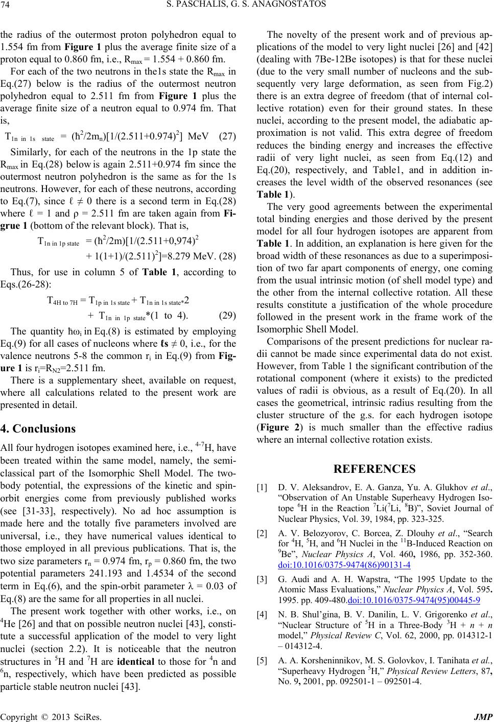 S. PASCHALIS, G. S. ANAGNOSTATOS 74 the radius of the outermost proton polyhedron equal to 1.554 fm from Figure 1 plus the average finite size of a proton equal to 0.860 fm, i.e., Rmax = 1.554 + 0.860 fm. For each of the two neutrons in the1s state the Rmax in Eq.(27) below is the radius of the outermost neutron polyhedron equal to 2.511 fm from Figure 1 plus the average finite size of a neutron equal to 0.974 fm. That is, T1n in 1s state = (ћ2/2mn)[1/(2.511+0.974)2] MeV (27) Similarly, for each of the neutrons in the 1p state the Rmax in Eq.(28) below is again 2.511+0.974 fm since the outermost neutron polyhedron is the same as for the 1s neutrons. However, for each of these neutrons, according to Eq.(7), since ℓ ≠ 0 there is a second term in Eq.(28) where ℓ = 1 and ρ = 2.511 fm are taken again from Fi- grue 1 (bottom of the relevant block). That is, T1n in 1p state = (ћ2/2m)[1/(2.511+0,974)2 + 1(1+1)/(2.511)2]=8.279 MeV. (28) Thus, for use in column 5 of Table 1, according to Eqs.(26-28): T4H to 7H = T1p in 1s state + T1n in 1s state*2 + T1n in 1p state*(1 to 4). (29) The quantity ћωi in Eq.(8) is estimated by employing Eq.(9) for all cases of nucleons where ℓs ≠ 0, i.e., for the valence neutrons 5-8 the common ri in Eq.(9) from Fig- ure 1 is ri=RN2=2.511 fm. There is a supplementary sheet, available on request, where all calculations related to the present work are presented in detail. 4. Conclusions All four hydrogen isotopes examined here, i.e., 4-7H, have been treated within the same model, namely, the semi- classical part of the Isomorphic Shell Model. The two- body potential, the expressions of the kinetic and spin- orbit energies come from previously published works (see [31-33], respectively). No ad hoc assumption is made here and the totally five parameters involved are universal, i.e., they have numerical values identical to those employed in all previous publications. That is, the two size parameters rn = 0.974 fm, rp = 0.860 fm, the two potential parameters 241.193 and 1.4534 of the second term in Eq.(6), and the spin-orbit parameter λ = 0.03 of Eq.(8) are the same for all properties in all nuclei. The present work together with other works, i.e., on 4He [26] and that on possible neutron nuclei [43], consti- tute a successful application of the model to very light nuclei (section 2.2). It is noticeable that the neutron structures in 5H and 7H are identica l to those for 4n and 6n, respectively, which have been predicted as possible particle stable neutron nuclei [43]. The novelty of the present work and of previous ap- plications of the model to very light nuclei [26] and [42] (dealing with 7Be-12Be isotopes) is that for these nuclei (due to the very small number of nucleons and the sub- sequently very large deformation, as seen from Fig.2) there is an extra degree of freedom (that of internal col- lective rotation) even for their ground states. In these nuclei, according to the present model, the adiabatic ap- proximation is not valid. This extra degree of freedom reduces the binding energy and increases the effective radii of very light nuclei, as seen from Eq.(12) and Eq.(20), respectively, and Table1, and in addition in- creases the level width of the observed resonances (see Table 1). The very good agreements between the experimental total binding energies and those derived by the present model for all four hydrogen isotopes are apparent from Table 1. In addition, an explanation is here given for the broad width of these resonances as due to a superimposi- tion of two far apart components of energy, one coming from the usual intrinsic motion (of shell model type) and the other from the internal collective rotation. All these results constitute a justification of the whole procedure followed in the present work in the frame work of the Isomorphic Shell Model. Comparisons of the present predictions for nuclear ra- dii cannot be made since experimental data do not exist. However, from Table 1 the significant contribution of the rotational component (where it exists) to the predicted values of radii is obvious, as a result of Eq.(20). In all cases the geometrical, intrinsic radius resulting from the cluster structure of the g.s. for each hydrogen isotope (Figure 2) is much smaller than the effective radius where an internal collective rotation exists. REFERENCES [1] D. V. Aleksandrov, E. A. Ganza, Yu. A. Glukhov et al., “Observation of An Unstable Superheavy Hydrogen Iso- tope 6H in the Reaction 7Li(7Li, 8B)”, Soviet Journal of Nuclear Physics, Vol. 39, 1984, pp. 323-325. [2] A. V. Belozyorov, C. Borcea, Z. Dlouhy et al., “Search for 4H, 5H, and 6H Nuclei in the 11B-Induced Reaction on 9Be”, Nuclear Physics A, Vol. 460, 1986, pp. 352-360. doi:10.1016/0375-9474(86)90131-4 [3] G. Audi and A. H. Wapstra, “The 1995 Update to the Atomic Mass Evaluations,” Nuclear Physics A, Vol. 595. 1995. pp. 409-480.doi:10.1016/0375-9474(95)00445-9 [4] N. B. Shul’gina, B. V. Danilin, L. V. Grigorenko et al., “Nuclear Structure of 5H in a Three-Body 3H + n + n model,” Physical Review C, Vol. 62, 2000, pp. 014312-1 – 014312-4. [5] A. A. Korsheninnikov, M. S. Golovkov, I. Tanihata et al., “Superheavy Hydrogen 5H,” Physical Review Letters, 87, No. 9, 2001, pp. 092501-1 – 092501-4. C opyright © 2013 SciRes. JMP 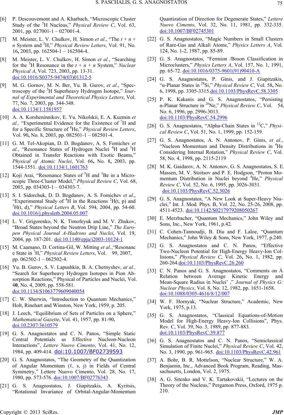 S. PASCHALIS, G. S. ANAGNOSTATOS 75 [6] P. Descouvemont and A. Kharbach, “Microscopic Cluster Study of the 5H Nucleus,” Physical Review C, Vol. 63, 2001, pp. 027001-1 – 027001-4. [7] M. Meister, L. V. Chulkov, H. Simon et al., “The t + n + n System and 5H,” Physical Review Letters, Vol. 91, No. 16, 2003, pp. 162504-1 – 162504-4. [8] M. Meister, L. V. Chulkov, H. Simon et al., “Searching for the 5H Resonance in the t + n + n Syste m, ” Nuclear Physical A, Vol. 723, 2003, pp. 13-31. doi:10.1016/S0375-9474(03)01312-5 [9] M. G. Gornov, M. N. Ber, Yu. B. Gurov, et al., “Spec- troscopy of the 5H Superheavy Hydrogen Isotope,” Jour- nal of Experimental and Theoretical Physics Letters, Vol. 77, No. 7, 2003, pp. 344-348. doi:10.1134/1.1581957 [10] A. A. Korsheninnikov, E. Yu. Nikolskii, E. A. Kuzmin et al., “Experimental Evidence for the Existence of 7H and for a Specific Structure of 8He,” Physical Review Letters, Vol. 90, No. 8, 2003, pp. 082501-1 – 082501-4. [11] G. M. Tel-Akopian, D. D. Bogdanov, A. S. Fomichev et al., “Resonance States of Hydrogen Nuclei 4H and 5H Obtained in Transfer Reactions with Exotic Beams,” Physical of Atomic Nuclei, Vol. 66, No. 8, 2003, pp. 1544-1551. doi:10.1134/1.1601763 [12] Koji Arai, “Resonance States of 5H and 5Be in a Micro- scopic Three-Cluster Model,” Physical Revie w C, Vol. 68, 2003, pp. 034303-1 – 034303-7. [13] S. I. Sidorchuk, D. D. Bogdanov, A. S. Fomichev et al., “Experimental Study of 4H in the Reactions 2H(t, p) and 3H(t, d),” Physical Letters B, Vol. 594, 2004, pp. 54-60. doi:10.1016/j.physletb.2004.05.007 [14] L. V. Grigorenko, N. K. Timofeyuk and M. V. Zhukov, “Broad States beyond the Neutron Drip Line,” The E uro- pen Physical Journal A-Hadrons and Nuclei, Vol. 19, 2004, pp. 187-201. doi:10.1140/epja/i2003-10124-1 [15] M. Caamano, D. Cortina-Gil, W. Mitting et al.,“Resonanc e State in 7H,” Physical Review Letters, Vol. 99, 2007, pp. 062502-1 – 062502-4. [16] Yu. B. Gurov, S. V. Lapushkin, B. A. Chernyshev, at al., “Search for Superheavy Hydrogen Isotopes in Pion Ab- sorption Reactions,” Physical of Particles and Nuclei, Vol. 40, No. 4, 2009, pp. 558-581. doi:10.1134/S1063779609040054 [17] C. W. Sherwin, “Introduction to Quantum Mechanics,” Holt, Rinehart and Winston, New York, 1959, p. 205. [18] J. Leech, “Equilibrium of Sets of Particles on a Sphere,” Mathematical Gazette, Vol. 41, 1957, pp. 81-90. doi:10.2307/3610579 [19] G. S. Anagnostatos and C. N. Panos, “Simple Static Central Potentials as Effective Nucleon-Nucleon Interactions”, Lettere Nuovo Cimento, Vol. 41, No. 12, 1984, pp. 409-414. doi:10.1007/BF02739593 [20] G. S. Anagnostatos, “The Geometry of the Quantization of Angular Momentum (ℓ, s, j) in Fields of Central Symmetry,” Lettere Nuovo Cimento, Vol. 28, No. 17, 1980, pp. 573-576. doi:10.1007/BF02776343 [21] G. S. Anagnostatos, J. Giapitzakis, A. Kyritsis, “Rotational Invariance of Orbital-Angular-Momentum Quantization of Direction for Degenerate States,” Lettere Nuovo Cimento, Vol. 32, No. 11, 1981, pp. 332-335. doi:10.1007/BF02745301 [22] G. S. Anagnostatos, “Magic Numbers in Small Clusters of Rare-Gas and Alkali Atoms,” Physics Letters A, Vol. 124, No. 1-2, 1987, pp. 85-89. [23] G. S. Anagnostatos, “Fermion /Boson Classification in Microclusters,” Physics Letters A, Vol. 157, No. 1, 1991, pp. 65-72. doi:10.1016/0375-9601(91)90410-A [24] G. S. Anagnostatos, P. Ginis, and J. Giapitzakis, “α-Planar States in 28Si,” Physical Review C, Vol. 58, No. 6, 1998, pp. 3305-3315.doi:10.1103/PhysRevC.58.3305 [25] P. K. Kakanis and G. S. Anagnostatos, “Persisting α-Planar Structure in 20Ne,” Physical Re view C, Vol. 54, No. 6, 1996, pp. 2996-3013. doi:10.1103/PhysRevC.54.2996 [26] G. S. Anagnostatos, “Alpha-Chain States in 12C,” Physi- cal Review C, Vol. 51, No. 1, 1999, pp. 152-159. [27] G. S. Anagnostatos, A. N. Antonov, P. Ginis, et al., “Nucleon Μomentum and Density Distributions in 4He Considering Internal Rotation,” Physical Review C, Vol. 58, No. 4, 1998, pp. 2115-2119 [28] M. K. Gaidarov, A. N. Antonov, G. S. Anagnostatos, S. E. Massen, M. V. Stoitsov and P. E. Hodgson, “Proton Mo- mentum Distribution in Nuclei beyond 4He,” Physical Review C, Vol. 52, No. 6, 1995, pp. 3026-3031. doi:10.1103/PhysRevC.52.3026 [29] G. S. Anagnostatos, “A New Look at Super-Heavy Niu- clei,” Int. J. Mod. Phys. B, Vol. 22, No. 25-26, 2008, pp. 4511-4523. doi:10.1142/S0217979208050267 [30] E. Merzbacher, “Quantum Mechanics,” John Wiley and Sons, Inc., New York, 1961, p.42. [31] C. Cohen-Tannoudji, B. Diu and F. Laloe, “Quantum Mechanics,” John Wiley & Sons, New York, 1977, p.240. [32] G. S. Anagnostatos and C. N. Panos, “Effective Two-Nucleon Potential for High-Energy Heavy-Ion Col- lisions,” Physical Review C, Vol. 26, No. 1, 1982, pp. 260-264.doi:10.1103/PhysRevC.26.260 [33] C. N. Panos and G. S. Anagnostatos, “Comments on Á Relation between Average Kinetic Energy and Mean-Square Radius in Nuclei’ ,” Journal of Physics G: Nuclear Physics, Vol. 8, No. 12, 1982, pp. 1651-1658. doi:10.1088/0305-4616/8/12/007 [34] W. F. Hornyak, “Nuclear Structure,” Academic, New York, 1975, p.13. [35] G. S. Anagnostatos, “Classical Equations-of-Motion Model for High-Energy Heavy-Ion Collisions”, Phys. Rev. C, Vol. 39, No. 3, 1989, pp. 877-883. doi:10.1103/PhysRevC.39.877 [36] G. S. Anagnostatos and C. N. Panos, “Semiclassical Simulation of Finite Nuclei,” Physical Review C, Vol. 42, No. 3, 1990, pp. 961-965. doi:10.1103/PhysRevC.42.961 [37] A. Bohr, B. R. Mottelson, “Nuclear Structure,” W. A. Benjamin, Inc., Advanced Book Program, Reading, Mas- sachusetts, London, Vol. 2, 1975. [38] A. G. Sitenko and V. K. Tartakovskii, “Lectures on the Theory of the Nucleus,” Pergamon Press, Oxford, 1975 p. 210. C opyright © 2013 SciRes. JMP  S. PASCHALIS, G. S. ANAGNOSTATOS Copyright © 2013 SciRes. JMP 76 [39] D. J. Rowe, “Nuclear Collective Motion (Models and Theory)”, Methuen and Co. Ltd., 11 New Fetter Lane, London EC4, 1970, p.78. [40] G. S. Anagnostatos, “Intrinsic-collective coupling in 6He and 8He,” In: Yu,E. Penionzhkevich and R. Kalpakchieva, Eds., Proceedings of the International Conference. on Ex- otic Nuclei, Foros, Crimea, 1-5 October, 1991. World Scientific, London, 1993, p. 104. [41] C. W. de Jager, H. de Vries, and C. de Vries, “Nuclear Charge and Momentum Distributions,” Atomic Data and Nuclear Data Tables, Vol. 14, No. 5-6, 1974, 479-665. doi:10.1016/S0092-640X(74)80002-1 [42] G. S. Anagnostatos, “Symmetry Description of the Independent Particle Model,” Lettere Nuovo Cimento, Vol. 29, No. 6, 1980, pp. 188-192. doi:10.1007/BF02743377 [43] J. Giapitzakis, “Συμμετρίες στην Πυρηνική Ύλη και στους Σ Υπερπυρήνες,” Ph.D. Dissertation, University of Patras, General Section, Patras, Greece, 2003. [44] G. S. Anagnostatos, “On the Possible Stability of Tetra- neutrons and Hexaneutrons,” International Journal of Modern Physics E, Vol. 17, No. 8, 2008, pp. 1557-1575.doi:10.1142/S0218301308010568  S. PASCHALIS, G. S. ANAGNOSTATOS 77 Supplementary sheet Calculations of Table1 concerning the manuscript: Ground state of 4-7H considering internal collective rotation Coordinates of all nucleon average positions appearing in Fig.2 in units Fermi For their identification the numbering here is the same as in the figure. (3΄) 0.000, 0.000, 1.554 (1) 0.974 cos450, 0.974 cos450, 0.000 (2) - 0.974 cos450, - 0.974 cos450, 0.000 (5) 0.000, 2.511, 0.000 (6) 0.000, -2.511, 0.000 (7) 2.511, 0.000, 0.000 (8) -2.511, 0.000, 0.000 Distances among all nucleon average positions, dij, corresponding nucleon potential energies, Vij of Eq.(6), and frequency of appearance in Fig.2 (in Fermi). d ij Vij 4H 5H 6H 7H d1-2 = d1-5 = d1-7 = d2-6 = d2-8 = 1.948 7.2808 2 3 4 5 d1-6 = d1-8 = d2-5 = d2-7 = 3.273 0.6306 1 2 3 4 d1-3΄= d2-3΄ = 1.834 9.1281 2 2 2 2 d5-3΄= d6-3΄= d7-3΄= d8-3΄ = 2.953 1.1133 1 2 3 4 d5-6 = d7-8 = 5.022 0.0323 1 1 2 d5-7 = d5-8 = d6-7 = d6-8 = 3.551 0.3879 2 4 Col.3 4H:ΣijVij = 7.2808*2+0.6306*1+9.1281*2+1.1133*1 = 34.56 5H: 7.2808*3+0.6306*2+9.1281*2+1.1133*2+0.0323*1 = 43.62 6H: 7.2808*4+0.6306*3+9.1281*2+1.1133*3+0.0323*1+0.3879*2 = 53.42 7H: 7.2808*5+0.6306*4+9.1281*2+1.1133*4+0.0323*2+0.3879*4 = 63.25 Application of Eqs.(9) and (8) for an1p neutron state. Energies of Table1 in MeV ћωn1p = (ћ2/m)(n+3/2)/<ri2> = 41.444(1+3/2)/2.511^2 = 16.4327 VLiSi=λ( ћωi )2 /(h2/m)*ℓi si = 0.03(16.4327)2/(41.444)*1/2 = 0.0977 ≈ 0.10 Col.4: 4 H ΣiVLiSi = 0.10, 5H 0.10*2= 0 20, 6H 0.0977*3=0.29, 7H 0.0977*4=0.39 Total kinetic energy according to Eq.(7) as already applied via Eqs.(25) – (28) Col.5 T1p in 1s state = 5.349 MeV 4H: Σ<T>nm = 5.349+1.706*2+8.279 = 17.04 T1n in 1s state = 1.706 MeV 5H: 5.349+1.706*2+8.279*2 = 25.32 T1n in 1p state = 8.279 MeV 6H: 5.349+1.706*2+8.279*3 = 33.60 7H: 5.349+1.706*2+8.279*4 = 41.88 Internal collective rotation for each isotope according to Eqs.(20) and (18) Θrot = Σ ρi2 + 0.165Arot Col.8 Arot i1 4H: Θrot,z= 2r+r +4*0.165=2(0.974cos45)2+(2.511)2+(1.554)2+4*0.165=10.329 2 1z2 8z 5H: Θrot,z= 2r+2r 2 8 +5*0.165 =2(2.511cos45)2+(1.554)2+5*0.165 = 9.545 2 1z z 6H: Θrot,(1,-1,1) = 7H: Θrot,(1,-1,1)= (ρpoint(0, 2.511, 0), axis(1,-1,1)=2(2.050)2 +2*0.165 = 8.735 Erot = (ћ2/2m) 2(2 + 1)/2Θrot =124.332/ Θrot Col.11: 4H Erot = 12.04, 5H Erot = 13.03, 6H Erot =14.23, 7H Erot = 14.23 Total binding energy for each hydrogen isotope:EB=Σ ijVij - Σ<T>nm-Σ iVLiSi -ER Col.12: 4H EB=34.56-17.04+0.10-12.04=5.58 5H EB=43.62-25.32+0.20-13.03=5.47 : EB=53.42-33.60+0.29-14.24=5.87 7H: EB=63.25-41.88+0.39-14 .24=7.52 C opyright © 2013 SciRes. JMP
|