Advances in Pure Mathematics, 2013, 3, 430-437
http://dx.doi.org/10.4236/apm.2013.34061 Published Online July 2013 (http://www.scirp.org/journal/apm)
Quasi-Static Problem of Thermoelasticity for
Thermosensitive Infinite Circular Cylinder
of Complex Heat Exchange
Halyna Harmatij1, Marta Król2, Vasyl Popovycz1
1Pidstryhach Institute for Applied Problems of Mechanics and Mathematics National Academy of Sciences of Ukraine,
Lviv, Ukraine
2Faculty of Mathematics and Applied Physics, Rzeszow University of Technology, Rzeszow, Poland
Received January 20, 2013; revised March 10, 2013; accepted April 13, 2013
Copyright © 2013 Halyna Harmatij et al. This is an open access article distributed under the Creative Commons Attribution License,
which permits unrestricted use, distribution, and reproduction in any medium, provided the original work is properly cited.
ABSTRACT
Nonlinear nonstationary heat conduction problem for infinite circular cylinder under a complex heat transfer taking into
account the temperature dependence of thermophysical characteristics of materials is solved numerically by the method
of lines. Directing it to the Cauchy’s problem for systems of ordinary differential equations studied feature which takes
place on the cylinder axis. Taken into account the dependence on the temperature coefficient of heat transfer that the
different interpretation of its physical content makes it possible to consider both convective and convective-ray or heat
ray. Using the perturbation method, the corresponding thermoelasticity problem taking into account the temperature
dependence of mechanical properties of the material is construed. The influence of the temperature dependence of the
material on the distribution of temperature field and thermoelastic state of infinite circular cylinder made of titanium
alloy Ti-6Al-4V by radiant heat transfer through the outer surface has been analyzed.
Keywords: Thermoelastic State; Heat Transfer; Boundary Value Problem
1. Introduction
It is of interest to consider the condition of convective
heat transfer coefficient depending on the temperature of
heat transfer
 
t
t
tt 


0
c
S
tt
n






t 
Sn
S
. (1)
Here t—coefficient of thermal conductivity, which
depends on the temperature; c
t—temperature environ-
ment, which washes the body surface ; -external nor-
mal to the surface . That kind of heat transfer condi-
tions also considers heating or cooling the body by ra-
diation, or heat when carried out simultaneously by con-
vection and radiation. Thus the physical content of Equ-
ation (1) is quite different. For radiation heat transfer co-
efficient t

is called the coefficient of radiation heat
transfer, it has the same dimension as the coefficient of
convective heat transfer is:
 


22
cc
ttttt



 , (2)

—
Stefan-Boltzmann constance,

—coefficient of black-
ness. The coefficient

is the total coefficient of con-
vective heat transfer k

and coefficient of radiation


t 

kt
  
r

,,rz 
in the case of convective heat transfer beam
where

. (3)
Transient heat transfer body will be called convective
heat transfer with temperature depending on the heat
transfer coefficient. The mechanism of that heat transfer
is described by the Relation (1).
In the study of processes of heat conduction in solids,
which are shaped circular cylinder radius 0 using a cy-
lindrical coordinate system . If the temperature
is independent of

and (the case of axial symme-
try), the heat equation has the form:
z

 
—reduced rate of radiation,
0
1,0
tv
tt
rct rr
rr r

 
 (4)



 



ctwhere v
The solution of Equation (4) satisfies the boundary
condition of the third kind, the described types of heat
transfer are as follows:
—volumetric heat capacity.
C
opyright © 2013 SciRes. APM

H. HARMATIJ ET AL. 431



0,
t
tr
tt
r





0,0 c
trt 



0r

, (5)
and at satisfies the condition of boundedness of
solution, which is equivalent to the condition
0
m 0
tt
tr 

li
r



,0
. (6)
Besides, the solution of Equation (4) satisfies the ini-
tial condition
p
tr t, (7)
where
p
t
t t
r
—the initial temperature of the cylinder.
Thus, the mathematical model to determine the tem-
perature field in a circular cylinder has the form of non-
linear boundary value Problems (4)-(7).
For the convenience of calculations in constructing the
solution to the Problems (4)-(7) we pass to dimensionless
variables. To do this, take the temperature of the heating
medium c by counting the temperature 0, and radius
0 for the typical size. We introduce the dimensionless
temperature 0 and coordinate Ttt0
rr

. The
growth temperature
p
T denoted by TT, where
0
t
pp
Tt
 
,tct 
.
2. Preliminaries
Specifications of the material tv and heat
transfer coefficient are represented as:

t 
 
 
 
0
0
0
,
,
,
ttt
vvv
tT
ccT
tT







,,c
ct
 
(8)
where 000tv

 —basic coefficients that are relevant
dimension, and,
  
,,TcT T 
 
T
tv —functions that
describe the dependence of these characteristics on di-
mensionless temperature , and



1
vp
TcT


tp
 .
We introduce the dimensionless time

2
000 00 t
F
oa rac  

and Bios criterion’
00 0t
Bi r

 . That Problems (4)-(7) to increase the
temperature in the dimensionless quantity becomes a
 
1
tT
Tc


 





 ,0 1
T
T
Fo



, (9)




1, 1, TFo
TBiT




0
tc
TFoT



(10)

0
lim

0
tT
T 

, (11)
00 Fo
T

, (12)
where ccp TTT.
Nonlinear boundary value Problems (9)-(12) will be
solved numerically using the method of lines. We intro-
duce a uniform grid


;0,, 1
hi
ih iNhN 

 
01
in the interval

. The differential operator


1
tT
T 



 





, (13)
has been replaced by the difference operator [1] at the
points of the grid,1, 1
iiN




12, ,
1
iii
i
i
T

, (14) 



where

12, 1
2,
ii iii
hTTTh



 ,


,1iii
TTTh
 
 i , and the value

determined by the
formula
1
2
ii
it
TT






(15)
or


1
2
ti ti
i
TT 




h
. (16)
The difference operator (14) approximates the dif-
ferential operator (13) to the second order in .
We will approach these functions

,TT Fo  
ii
by
using the functions


,0,yyFoi N
ii , which are based
on Equation (9) satisfying the system of ordinary differ-
ential equations

11
12 112
d
d
1,
1, 1
i
ii ii
ii ii
ii
y
Fo
yy yy
hc hh
iN
 


 



 (17)






where

ccT


1
ivi
We construct the difference boundary condition for the
second-order approximation for N
.

 . The expan-
sion of these values in series Taylor in neighborhood of
the point

N


is written as follows:

   
1
2
2
,12
2
2
2
2
NN
N
NN
N
NN
Nt Nt
TT
h
ThT
TOh
h
TTOh

 




 








 


 

Then considering the differential Equation (9) at the
point

N


we receive

H. HARMATIJ ET AL. 432
 



 

  
2
2
2.
N
N
N
NN
t
T
TOh
T
Oh
Oh










 



 








12 ,
2
2
2
1
2
2
N N
N
NNN
tt
t
tN
tNt
T
Th
TT
T
Th
TT
ThT
TcT
Fo




 

 

 
 

 
































Hence, taking into account that
N
N
Ty, we obtain

12 ,
NN N
y

 


d2
d
NNN
NN
y
Fo h c


, (18)
where


1
1
N
c
T T
 
Bi T



 .
The difference analog of condition is constructed (11).
The values ,0 T

і 1

decompose in the Taylor series:

   
2
2
0
,
.
TO
h
Oh
 


2
,0 2
00
10
2
2
tt
ThT
h
TT



 









Then
  
 
 
 
00
2
2
0
T
TOh
TOh



















1,0
0
2
2
0
0
2
2
tt
t
tt
T
Th
TT
T
Th
TT


















 








(19)
In view of Equation (9) we write
  
t
tT
TTT
TcT
F
o



 







 



 . (20)
Since 0 lim 0
T






, then we have uncertainty
0
tTT







of type 0
0. We now turn to the border
and reveal uncertainty using the rule of de L’Hospitala,
we get

0
0
lim t
t
TTT
T


 





  


 


.


Thus from (20) we obtain
 
0
0
0
1
2
tTT
TcT
Fo









  



 

 . (21)
Taking into account (21), we write (19) as


2
1,0 0
0
4v
hT
TcT Oh
Fo






. (22)
Since the value of 0 approaches 0, then from (22)
we obtain the following differential equation at the point
Ty
0


0
1,0
d4
d
yy, (23)
F
ohc
 


where

.
00 v
ccT




Thus, we obtain the Cauchy problem for systems of
ordinary differential equations approximating the partial
derivatives of the space variables with the second-order
boundary-value Problems (8)-(11)

0
11 0
2
0
d4
d
yyy
Foc h
 , (24)
 

12 11121
2
d1,
d
1,1 ,
iiiii iiii
ii
yyy yy
Fo hc
iN
 

 






(25)
1
12
d2
d
NNN
NN NN
NN
yyy
Fo h ch
 










00
i
y
, (26)
. (27)
Thus, the dependence forms of the heat transfer co-
efficient


t 

t  , thermal conductivity t and volu-
metric heat capacity


ct
v of the selected material are
dependent on temperature, then we solve the system
numerically (24)-(27). As a result, we obtain the value
of temperature increase in grid points ,1,iN  
i along
the radius of the cylinder for a given time
F
o
,,
rr zz 
.
3. Thermoelastic State of a Cylinder
The thermoelastic cylinder state with the activity of the
found axisymmetric temperature field are defined by
three non-zero components of stress tensor




,
which in dimensionless form is rewritten as:
00
,,
,, 2
rr zz
to
Gt



 

0
G0t
,
where і

—supporting values of the shear mo-

H. HARMATIJ ET AL. 433
dulus and coefficient of linear thermal expansion.
However, they are expressed through the dimension-
less radial displacement
00to
u
urt

, so







*
1,
uu
T e
TT










1GT T







(28)
  


  
1,
T e
TT








1
uu
GT T T
 






(29)

    
*
e T

1
uu
GT TT




 
 







(30)
and satisfy the equation of balance
0





. (31)
Here
0
z
z
e
e


to
t 
, where
z
z
e—was the axial strain;



 




0
1
,d
12 1
T
t
GT T
GT T
TT









,
(
 
,,TTGT 

t—the function describing the de-
pendence of the Poisson coefficient of the linear thermal
expansion and modulus of the dimensionless temperature
increase. If we substitute the dependence (28)-(30) into
equilibrium Equation (31), we get the differential equa-
tion


  
, T






1u
Tuu
nTeTmT











 
 

(32)
where
  
 
  

 


 





ln 1,
1
1
TGTT
mTGT TGT
GT
nT GT T














1,
.
T
T
 
The solution of Equation (32), which satisfies the con-
dition of the limited movement of the cylinder axis,
found by perturbation [1-3] has the form of:
0
k
k
uu


, (33)
where








02
010
002
11 1
2
1
2nn
uc HHH
eHH





 


 






(34)







 
02
1
02
11
1
2
11
,1
2
k
kkn n
kk
e
ucH H
HHk



 



 



(35)




 

 

 

 
 
0
0
0
11
0
11
1
d
d
d
d
.
mm
mm
n
mm
kk
kk
k
HT
HT
Hn
Hf
uu
fTmT





 
 

 
 









 








,, According to (33) the thermal stress





 
0
,,,,
, is
found by the formulas:
p
pk kk
k
 
 


, (36)
where










0102
0
12
,
n
TH
GT c
HeTH












 (37)

 






 
11
,1,
pk
kknk
GT ceTHHk






 

(38)











0
01 2
0
12
12
,
n
TH
GT cTT
HevTH












 




 

(39)

H. HARMATIJ ET AL. 434




1
k
kk n
GT ceTHH









1
,1
kk




(40)


 

 


 



0
01
0
0
212
1,
n
GTT cTT
evTvTH



0
T H








 



(41)

  





1
0
1
21
k
kk
k
GTT ceT
TH




0
,1
n
T H
k












(42)
where







02
,
,, 1.
H
nk









10 k

0
k
ek


2
12
1
2
T
HH






The sustainable integration ck and parts of
the development of axial strain determine the
conditions on the outer surface 10
k 


1
0
d0
k 
 
and relations
for unmounted ends of the cylinder

, by
solving system of linear equations


,0
kk
B kAX , (43)
where




 




 
 









1
1
1
1
1
11 12
21 22
1112 11
21
0
22
0
10 111
20 1
0
111
0
21
0
,,
1,
2d
1
,
k
kk
k
n
kk
kk
c
aa
e
aa
aa H
aGTT
aGTT
bHH
bGT T
bH
bGTTH








1
2
0
0
d
d
d.
k
k
n
b
b
TH
TH



 




 
























AX







B
Here


111 111
1
1,,1 2 ,TGGT.

 


 
0e

For fixed ends of the cylinder we have .

If the thermomechanical properties of the material the
cylinder does not depend on temperature, then transfer
and thermal stresses are calculated by the formulas:

0
1,d ,
1
iti
iii
i
uTFoc








 (44)
 
2
0
11
,d ,
112
i
iti
ii iii
ii
GTFone




 
 





 







(45)
 

2
0
11,d ,
1
1,
12
i
iti
iii
i
iii
i
GTFoTFo
ne




  


















(46)
  
1
2121 ,,
12 1
i
ii
iii iitii
ii
Gce TFo




 



 
 




(47)
where

1
2
10
13 ,d
1
iti
ii
i
cTFo







,






1
2
2
10
0
111 2,d
12
ii
ti
ii
i
eTFo










 ,


,TFo 
*
,G 

trr
300 Kt
t
i—increase of temperature in the cylinder for
constant thermophysical characteristics; i—steel
coefficient of linear thermal expansion and modulus ta-
ken at the initial or maximum temperature, or mean inte-
gral value of the selected temperature range.
4. Numerical Study
This section investigated the temperature field and ther-
moelastic state of thermosensitive infinite circular cylin-
der. Radiant heat exchange with the environment at a
temperature c is due to the surface 0 of the cylin-
der, which is free from power loads. In that case, the ra-
diant heat exchange has been formed to convective heat
transfer coefficient in the form of (2). The initial tem-
perature of the cylinder is p. The medium tem-
perature c is equal to 1100 K and it is selected by sup-
porting. Titanium alloy Ti-6Al-4V taken by the material.
Temperature dependence of thermal and mechanical
properties of the alloy are the form [4] in the temperature
range from 300 K to 1100 K.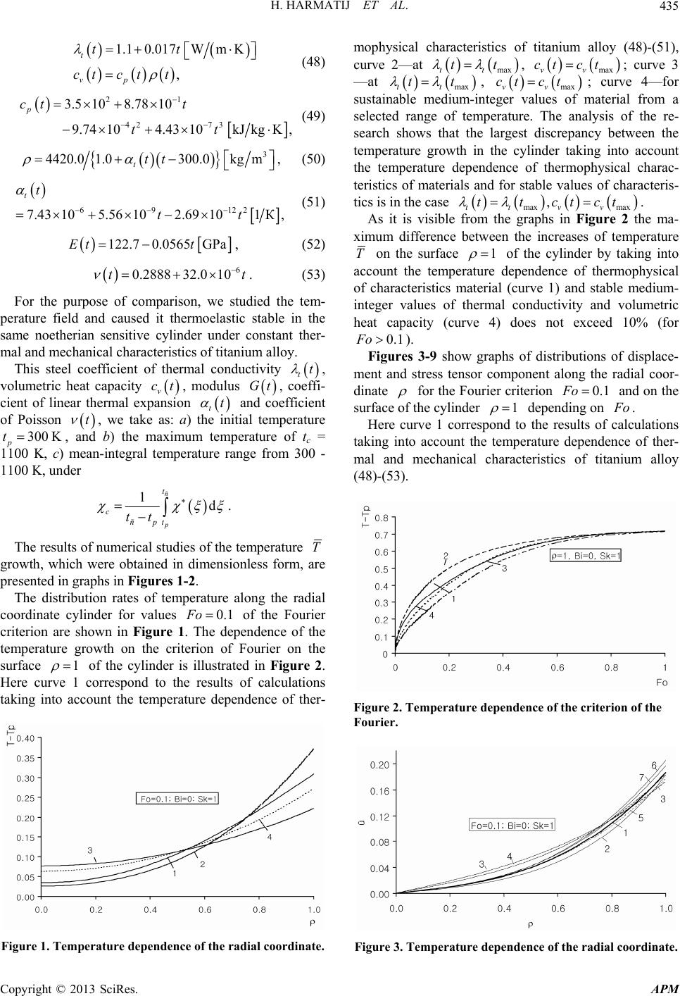

H. HARMATIJ ET AL. 435
 

1.1 0.017
,
t
vp
tt
ct ctt




Wm K


(48)


3kJ kgK ,

21
42 7
3.510 8.7810
9.74104.43 10
p
ct t
tt


 
 

(49)

3
.0kgm



4420.0 1.0300
ttt
 

, (50)

122
101 К,tt


69
7.43 105.56 102.69
t

 
 
t 
(51)

122.7 0.0565 GEt tPa
6
8832.010tt


, (52)

0.28  . (53)
For the purpose of comparison, we studied the tem-
perature field and caused it thermoelastic stable in the
same noetherian sensitive cylinder under constant ther-
mal and mechanical characteristics of titanium alloy.
This steel coefficient of thermal conductivity


t 

ct

Gt
300 K
t,
volumetric heat capacity v, modulus , coeffi-
cient of linear thermal expansion and coefficient
of Poisson , we take as: a) the initial temperature
p, and b) the maximum temperature of tc =
1100 K, c) mean-integral temperature range from 300 -
1100 K, under

tt


t 
t

1d
n
p
t
np t
ctt







.
The results of numerical studies of the temperature T
0.1Fo 
1
growth, which were obtained in dimensionless form, are
presented in graphs in Figures 1-2.
The distribution rates of temperature along the radial
coordinate cylinder for values of the Fourier
criterion are shown in Figure 1. The dependence of the
temperature growth on the criterion of Fourier on the
surface

 of the cylinder is illustrated in Figure 2.
Here curve 1 correspond to the results of calculations
taking into account the temperature dependence of ther-
Figure 1. Temperature dependence of the radial coordinate.
mophysical characteristics of titanium alloy (48)-(51),
curve 2—at


 
maxtt
tt  
 
vv
ct ct, max ; curve 3
—at


 
tt  maxtt,

 
ct ctmaxvv; curve 4—for
sustainable medium-integer values of material from a
selected range of temperature. The analysis of the re-
search shows that the largest discrepancy between the
temperature growth in the cylinder taking into account
the temperature dependence of thermophysical charac-
teristics of materials and for stable values of characteris-
tics is in the case

   
,ttct ct  
max maxtt vv
As it is visible from the graphs in Figure 2 the ma-
ximum difference between the increases of temperature
.
T1 on the surface


of the cylinder by taking into
account the temperature dependence of thermophysical
of characteristics material (curve 1) and stable medium-
integer values of thermal conductivity and volumetric
heat capacity (curve 4) does not exceed 10% (for
). 0.1Fo 
Figures 3-9 show graphs of distributions of displace-
ment and stress tensor component along the radial coor-
dinate

for the Fourier criterion and on the
surface of the cylinder
0.1Fo 
1
F
o.


depending on
Here curve 1 correspond to the results of calculations
taking into account the temperature dependence of ther-
mal and mechanical characteristics of titanium alloy
(48)-(53).
Figure 2. Temperature dependence of the criterion of the
Fourier.
Figure 3. Temperature dependence of the radial coordinate.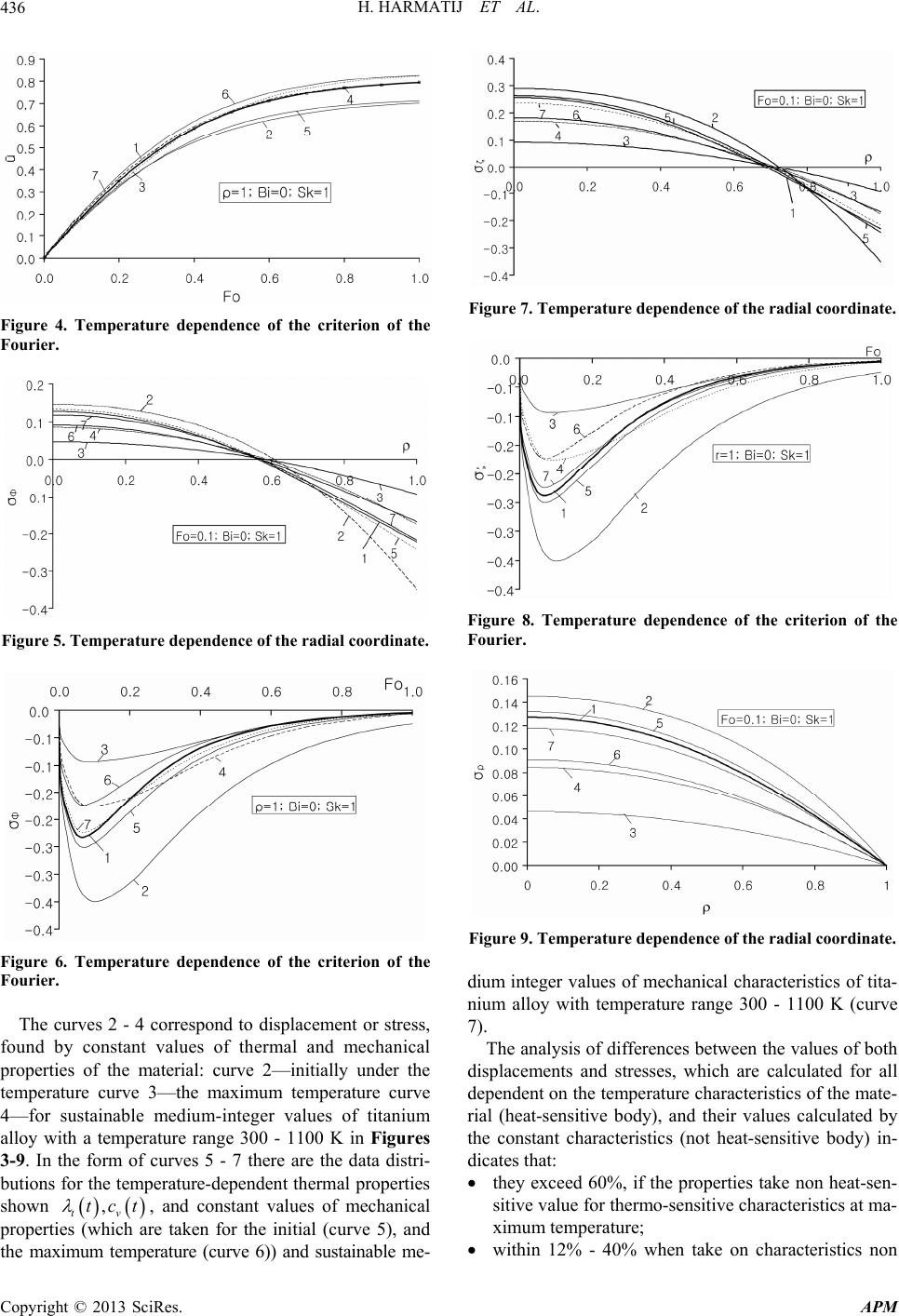

H. HARMATIJ ET AL. 436
Figure 4. Temperature dependence of the criterion of the
Fourier.
Figure 5. Temperature dependence of the radial coordinate.
Figure 6. Temperature dependence of the criterion of the
Fourier.
The curves 2 - 4 correspond to displacement or stress,
found by constant values of thermal and mechanical
properties of the material: curve 2—initially under the
temperature curve 3—the maximum temperature curve
4—for sustainable medium-integer values of titanium
alloy with a temperature range 300 - 1100 K in Figures
3-9. In the form of curves 5 - 7 there are the data distri-
butions for the temperature-dependent thermal properties
shown tv , and constant values of mechanical
properties (which are taken for the initial (curve 5), and
the maximum temperature (curve 6)) and sustainable me-
Figure 7. Temperature dependence of the radial coordinate.
Figure 8. Temperature dependence of the criterion of the
Fourier.
Figure 9. Temperature dependence of the radial coordinate.
dium integer values of mechanical characteristics of tita-
nium alloy with temperature range 300 - 1100 K (curve
7).
The analysis of differences between the values of both
displacements and stresses, which are calculated for all
dependent on the temperature characteristics of the mate-
rial (heat-sensitive body), and their values calculated by
the constant characteristics (not heat-sensitive body) in-
dicates that:
 they exceed 60%, if the properties take non heat-sen-
sitive value for thermo-sensitive characteristics at ma-
ximum temperature;
 
,tct 
 within 12% - 40% when take on characteristics non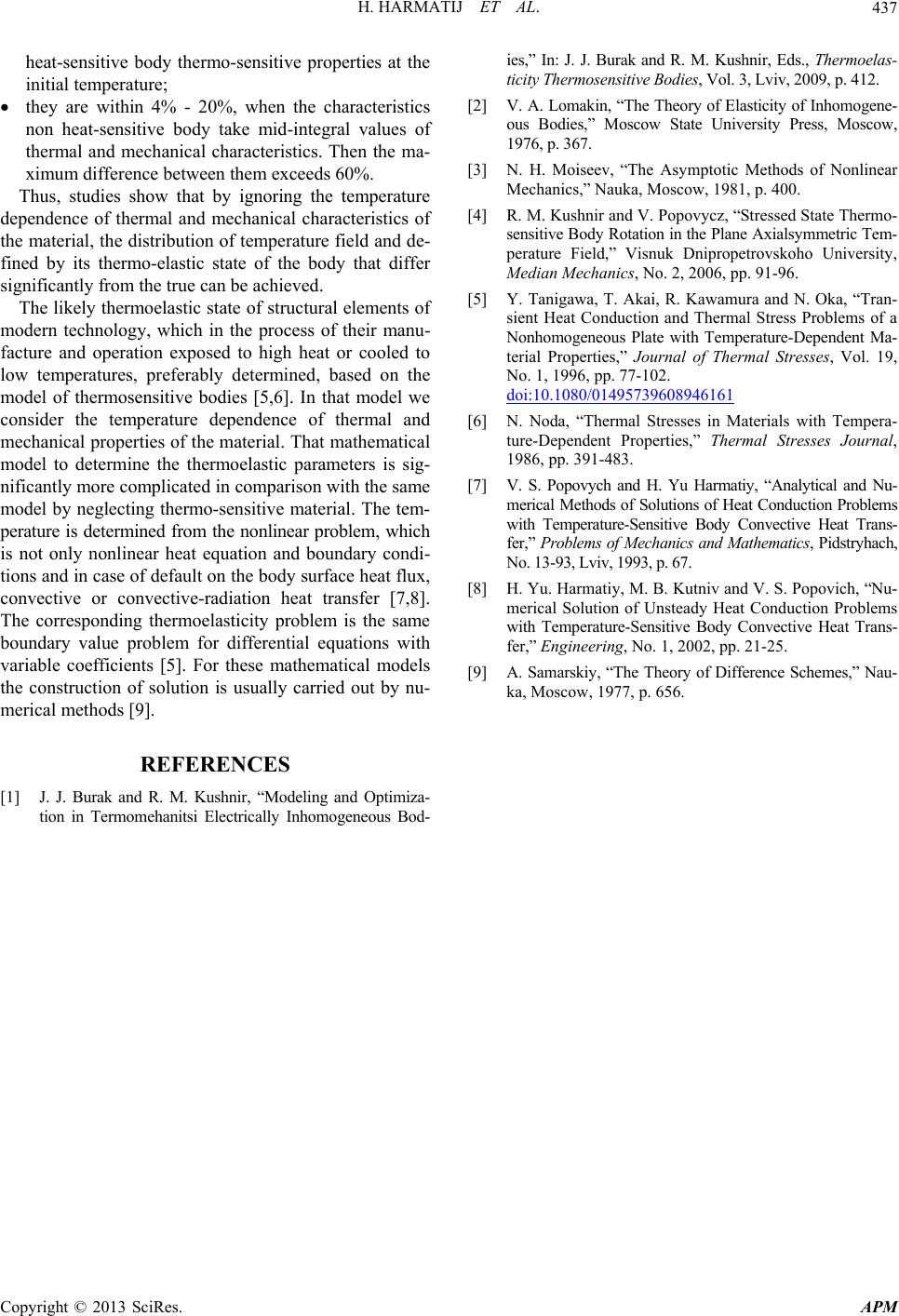

H. HARMATIJ ET AL. 437
heat-sensitive body thermo-sensitive properties at the
initial temperature;
 they are within 4% - 20%, when the characteristics
non heat-sensitive body take mid-integral values of
thermal and mechanical characteristics. Then the ma-
ximum difference between them exceeds 60%.
Thus, studies show that by ignoring the temperature
dependence of thermal and mechanical characteristics of
the material, the distribution of temperature field and de-
fined by its thermo-elastic state of the body that differ
significantly from the true can be achieved.
The likely thermoelastic state of structural elements of
modern technology, which in the process of their manu-
facture and operation exposed to high heat or cooled to
low temperatures, preferably determined, based on the
model of thermosensitive bodies [5,6]. In that model we
consider the temperature dependence of thermal and
mechanical properties of the material. That mathematical
model to determine the thermoelastic parameters is sig-
nificantly more complicated in comparison with the same
model by neglecting thermo-sensitive material. The tem-
perature is determined from the nonlinear problem, which
is not only nonlinear heat equation and boundary condi-
tions and in case of default on the body surface heat flux,
convective or convective-radiation heat transfer [7,8].
The corresponding thermoelasticity problem is the same
boundary value problem for differential equations with
variable coefficients [5]. For these mathematical models
the construction of solution is usually carried out by nu-
merical methods [9].
REFERENCES
[1] J. J. Burak and R. M. Kushnir, “Modeling and Optimiza-
tion in Termomehanitsi Electrically Inhomogeneous Bod-
ies,” In: J. J. Burak and R. M. Kushnir, Eds., Thermoelas-
ticity Thermosensitive Bodies, Vol. 3, Lviv, 2009, p. 412.
[2] V. A. Lomakin, “The Theory of Elasticity of Inhomogene-
ous Bodies,” Moscow State University Press, Moscow,
1976, p. 367.
[3] N. H. Moiseev, “The Asymptotic Methods of Nonlinear
Mechanics,” Nauka, Moscow, 1981, p. 400.
[4] R. M. Kushnir and V. Popovycz, “Stressed State Thermo-
sensitive Body Rotation in the Plane Axialsymmetric Tem-
perature Field,” Visnuk Dnipropetrovskoho University,
Median Mechanics, No. 2, 2006, pp. 91-96.
[5] Y. Tanigawa, T. Akai, R. Kawamura and N. Oka, “Tran-
sient Heat Conduction and Thermal Stress Problems of a
Nonhomogeneous Plate with Temperature-Dependent Ma-
terial Properties,” Journal of Thermal Stresses, Vol. 19,
No. 1, 1996, pp. 77-102.
doi:10.1080/01495739608946161
[6] N. Noda, “Thermal Stresses in Materials with Tempera-
ture-Dependent Properties,” Thermal Stresses Journal,
1986, pp. 391-483.
[7] V. S. Popovych and H. Yu Harmatiy, “Analytical and Nu-
merical Methods of Solutions of Heat Conduction Problems
with Temperature-Sensitive Body Convective Heat Trans-
fer,” Problems of Mechanics and Mathematics, Pidstryhach,
No. 13-93, Lviv, 1993, p. 67.
[8] H. Yu. Harmatiy, M. B. Kutniv and V. S. Popovich, “Nu-
merical Solution of Unsteady Heat Conduction Problems
with Temperature-Sensitive Body Convective Heat Trans-
fer,” Engineering, No. 1, 2002, pp. 21-25.
[9] A. Samarskiy, “The Theory of Difference Schemes,” Nau-
ka, Moscow, 1977, p. 656.