 Journal of Modern Physics, 2013, 4, 930-939 http://dx.doi.org/10.4236/jmp.2013.47125 Published Online July 2013 (http://www.scirp.org/journal/jmp) Mathematical Derivation of Angular Momenta in Quantum Physics Daniel Grucker Université de Strasbourg-CNRS, Strasbourg, France Email: d.grucker@unistra.fr Received April 24, 2013; revised May 27, 2013; accepted June 26, 2013 Copyright © 2013 Daniel Grucker. This is an open access article distributed under the Creative Commons Attribution License, which permits unrestricted use, distribution, and reproduction in any medium, provided the original work is properly cited. ABSTRACT For a two-dimensional complex vector space, the spin matrices can be calculated directly from the angular momentum commutator definition. The 3 Pauli matrices are retrieved and 23 other triplet solutions are found. In the three-dimen- sional space, we show that no matrix fulfills the spin equations and preserves the norm of the vectors. By using a Clif- ford geometric algebra it is possible in the four-dimensional spacetime (STA) to retrieve the 24 different spins 1/2. In this framework, spins 1/2 are rotations characterized by multivectors composed of 3 vectors and 3 bivectors. Spins 1 can be defined as rotations characterized by 4 vectors, 6 bivectors and 4 trivectors which result in unit multivectors which preserve the norm. Let us note that this simple derivation retrieves the main spin properties of particle physics. Keywords: Quantum Systems; Spin 1/2; Spin 1; Particle Physics, Spacetime Algebra 1. Introduction 0101 0 ,, 1000 1 xy z i i The spin of particles was discovered by Wolfgang Pauli toward the end of 1924 (see Fröhlich’s paper for an up- to-date discussion of spins [1]). In quantum mechanics textbooks, the matrix representation of spin is obtained from the commutator general definition of the angular momentum: , yz JiJ , yz x (1) JiJ (2) , xy JiJ 2222 (3) These 3 equations are called the spin equations. The general theory of quantum angular momenta [2] uses the operator yz JJJ, the two shift op- erators x , x JiJ J JiJ and the positive ei- genvalue 1jj of J2. The values for j are 0,12,1,32, 2,. For j = 0, the spin space is of dimen- sion 1 and reduced to a scalar equal to zero. For j = 1/2, the spin space is of dimension 2 and the matrix represen- tation is given by 11 22 1 ,, 2 xy JJ yz z J (4) where i are the Pauli matrices: ,, (5) These three J matrices describe the so called spin 1/2 quantum system. The aim of this work is to address two questions: can the Pauli matrices or more generally any spin system be retrieved directly from the angular momentum definition and are the 3 Pauli matrices the only 2-dimensional quan- tum angular momenta? 2. Properties of the Minimum-Dimension Quantum Spin System The smallest quantum angular momentum is of dimen- sion 3 because there are 3 elements yz JJ . As quan- tum mechanic acts on complex vector spaces, the mini- mum dimension is a two-dimensional complex space or a four-dimensional real space with two elements multiplied by 1i which is different from a true four-dimen- sional real space. 2.1. Matrix Description The two components of the vectors of such a space can be written as 123 4 , ix xix 1 2 12 1 34 2 ie ie i i xx r xx r or in matrix notation: (6) C opyright © 2013 SciRes. JMP  D. GRUCKER 931 which corresponds to an ordered set of four real ele- ments. An operator in such a vector space is given by ij a 12 34 viv viv 2222 1234 vvv a real 2 2 matrix multiplied by a complex number α. It can be noticed that the two parts of α pro- vide the information about the position of i in the four real number set aij. Quantum mechanics only studies operators which pre- serve the norm, and in two dimensions this is written as: 1211 12 342122 vivaa vivaa (7) with 2 2 2 2 1234 v v v vv (8) The solution is: 2 22 11 21 1aa (9) 22 12 212 1aa 1221 220aa †1MM 2 (10) 11 aa (11) which corresponds to (12) This result can be easily generalized to quantum vector spaces of any dimension. We see that αM is not a unitary matrix because it fulfills only one of the two conditions of a unitary matrix †† 1UU 11 12 21 22 kk kk kk UU . This implies that quantum operators need not be unitary in order to pre- serve the norm in the vector space contrary to frequently held views. The problem studied was to find the 12 real elements of the three following matrices: J (13) with the three αk complex numbers for k = x, y, z. The subscripts have presently nothing to do with the space coordinates. From Equation (1), it follows that the matrix Jz is: 11 12 21 22 xy zz zz 12212112 yxy 12 2211 xyy 21 1122 xyy zz z Ji (14) with 11 zx 1212 1122 zyxx zyxx 2121 2211 2221121221 zxyxy which shows that 2211 . Mor generally it is well known that the commutator of two matrices results in a matrix with a null trace. As Jx and Jy are defined by a commutator, we also have 22 11 x 11 yy and 22 . From Equation (2) it follows that the matrix Jx is: 11 12 21 22 yz x x J x i (15) with 1221 111121121221 11 2 12 21 22 2 yyxy xyxy xyy 2 12211211 11 12 22 1112 21 24 42 yx yyx xyyy 2 21 12211111 21 22 1112 21 24 42 yx yyx xyyy 12 21111112212112 22 2 12 21 22 2 yyxy xyxy xyy From Equation (3) it follows that the matrix Jy has the same expression as Jx just by exchanging y and x. Calcu- lating 21 121221 yxy by eliminating x11 gives a relation between the Jy elements: 2224 1112211221 42 40yyy yy (16) As Jy is a quantum operator we have the general con- straints given by Equations (9)-(11) on the Jy elements: 22 11 212 1 x yy K (17) 22 12 112 1 x yy K (18) 11 12210yy y 0y0yy 11 0y (19) where K is a positive real constant. Equation (19) implies that or . 1112 21 For , Equations (17) and (18) imply that 22 21 12,yyK 21 12 yy 11 0y therefore . and 21 12 yy, Equation (16) gives For 12 2yi and we obtain the second Pauli matrix 1 0 0 2 yy i JJ i (20) or its opposite 2yy . J 11 0yFor and 21 12 yy Equation (16) gives 12 2yi and we obtain the first Pauli matrix: 3 01 10 2 yx JJ 43yy (21) or its opposite J 11 0y The case permits to calculate the constant 24. Copyright © 2013 SciRes. JMP  D. GRUCKER 932 For and , Equation (16) gives 11 0y 222 21 12 yy 224 12 4 0y 11 12 42yy and using Equation (18) 222 11 12 we obtain 4yy2 12 0y and 11 2y which gives the third Pauli matrix: 5yz JJ 10 01 2 65yy (22) or its opposite J . The 6 Jyk matrices are Jy, −Jy , Jx, −Jx, Jz, −Jz. The norm preservation and the null trace constraints applied to Jx give the 6 different Jxk matrices Jx, −Jx, iJy, −iJy, Jz, −Jz which fulfill the angular momentum criteria. Let us note that all are real matrices. All the matrix triplets which fulfill the angular mo- mentum definition in the two-dimensional complex vec- tor space are obtained with Equation (14). For each Jxk there are 6 Jyk which gives 36 possibilities for Jz which fulfill the 3 Equations (1)-(3). Out of these 36 possibili- ties only 24 give a nonzero matrix. Obtaining the 24 so- lutions is straightforward and only two examples will be given explicitly. The first one is the well-known Pauli spin 1/2 matrices: 11 01 0 ,, 10 0 22 xy i JJ i 1 1 0 0 1 2 z J (23) and the second example is less conventional: 1313 13 01 01 ,, 10 10 22 xy JJ 0 0 2 z i J i 1 0 0 1 Z J (24) It can easily be verified that these 3 matrices fulfill the 3 angular momentum definitions given by Equations (1)- (3). The 24 solutions show that the elements of the spin 1/2 matrices can take only four values (−1, −i, i, +1) times ħ/2 and the corresponding real matrices: 0101 ,, 101 0 XY JJ (25) Let us note that: 22 1, XY JJ 2 1, 1 Z J (26) and †† 1, 1 Xx YY JJ JJ † , 1 ZZ JJ 2222 (27) which proves that all the solutions correspond to an op- erator which preserves the norm of the vectors in the two-dimensional space. The 24 solutions of the general definition of the angu- lar momenta for spin 1/2 are given in Table 1. The general treatment of angular momenta uses the operator yz JJJ. If we calculate this operator for the 24 solutions we find 22 1 3 4 I in 16 cases corresponding to the first two and last two rows of Table Table 1. The 24 solutions for spin 1/2 using matrices JX, JY, JZ, in ħ/2 units. J1(JX,iJY,JZ) J2(JX,−iJY,−JZ)J3(JX,JZ,−iJY) J4(JX,−JZ,iJY) J5(−JX,iJY,−JZ)J6(−JX,−iJY,JZ)J7(−JX,JZ,−iJY) J8(−JX,−JZ,iJY) J9(JY,JX,iJZ) J10(JY,−JX,−iJZ)J11(JY,JZ,−iJX) J12(JY,−JZ,iJX) J13(−JY,JX,−iJZ)J14(−JY,−JX,−iJZ) J15(−JY,JZ,iJX) J16(−JY,−JZ,−iJX) J17(JZ,iJY,−JX)J18(JZ,−iJY,JX)J19(JZ,JX,iJY) J20(JZ,−JX,−iJY) J21(−JZ,iJY,JX)J22(−JZ,−iJY,−JX) J23(−JZ,JX,−iJY) J24(−JZ,−JX,iJY) 1. This result is the well-known value obtained with Pauli matrices. In the other 8 cases (rows 3 and 4 of Ta- ble 1) we obtain 22 1 1 4 I kkxxkyykzz JJJ . We can associate the spin 1/2 with components Jkx, Jky and Jkz to the space coordinates in the laboratory frame (O,ux,uy,uz) to define the spin vector of a particle: uuu (28) 2.2. Dirac Equation It is well known [2] that the spin of a particle can be re- trieved using an equation which satisfies the special the- ory of relativity and quantum mechanics postulates, such as the Dirac equation. In Dirac’s book [3], the Pauli ma- trices are obtained from the commutation definition with the additional constraint: 2 222 4 xyz JJJ 0e e0 ia xia 2 222 1, 0 ,0 xxyyx xx mc (29) Owing to the fact that each observable has only two eigenvalues ħ/2 and −ħ/2. He obtained (30) and stated that the phase could be adequately chosen so as to obtain the three Pauli matrices. It is clear that Dirac did not consider non observable spins and he only took the 3 Pauli matrices as components of the spin vector. In his relativistic theory of the electron, he found that in order to obtain a linear wave equation it was necessary to introduce four 4 4 matrices solving the following equations: 1 1 0, 0 kk k kk I I (31) and the same relations obtained by permuting x,y and z. A solution given by Dirac to these four matrices was: (32) with k = x, y, z, which nowadays is referenced as the standard form. But it is well known that any set of ma- Copyright © 2013 SciRes. JMP  D. GRUCKER 933 trices obtained with: †† U UandUU †† 1UU (33) where U is any unitary matrix , is also a solution to Equations (31). It can be shown that for a homogeneous magnetic field, the energy of the interac- tion of the intrinsic momentum with the magnetic field is UU 0 2 s q EB m (34) and the spin definition can also be retrieved as 1 2 S (35) where is the spin vector defined by the 3 Pauli ma- trices as in the non relativistic case. Dirac’s equation has to be discussed more precisely only when time evolution is introduced. An important question is why does the general treat- ment of quantum angular momentum give only one solu- tion? This comes from the definition of 2222 yz JJJ 1,, which is a dot product and not the matrix product of two angular momentum components. This definition intro- duces some constraints which permit to eliminate the solutions where J2 < 0, but by taking only the positive values of j, also eliminates the negative components in the combination of the Pauli matrices. Therefore only the solution yz J is obtained. 3. Angular Momenta for 3-Dimensional Quantum System If we consider the extension to three dimensions, a vector has now 3 components and any quantum operator is de- scribed by a real 3 3 matrix multiplied by a complex number 1 2 3 00 00 00 . We can choose a basis for the vector space where one angular momentum is diagonal. If we take the z direction for this, the angular momentum is: z J J (36) where the λk are three complex numbers. As the angular momenta are defined by Equations (1)-(3) which correspond to non commuting matrices the trace of the 3 angular momentum matrices Jx, Jy, Jz is null. If we suppose that in the same basis and for the most general case yij where βij are complex numbers, we obtain according to Equation (2): 12 21 21 21 31 313232 0 10 x Ji 13 31 23 32 0 (37) and Equation (3) gives: 2 2 2 122113 31 2 2 21 2123 32 22 31 313232 1 0 0 0 y J (38) and Equation (1): 4 1 ij J (39) 3 3 11122112133113 3 3 2212212123 3223 33 3313 3131233232 12133231 23 123 131223213 22 32 2321 131231231 21233132 1 3 1 2 2 2 2 2 2 23 31213212231132 3231121 32 1 231 2 2 2 (40) 0 To find the angular momenta, Equation (39) must be equal to Equation (36). There are several solutions ob- tained from the non diagonal Jz matrix elements equal to zero. If 1331 2 , then 1. For 1 we obtain a set of three matrix solutions to the spin equation: 12 2 23 12 2 23 12 2 23 12 2 23 0i 0 10 0i 00 0,0i, 2 00 1 i 00 2 00 0 2 00 2 zx y JJ J , (41) For 1 the sign of Jz and Jx is changed but Jy is unchanged. If 12 23 we retrieve the con- ventional matrices for a spin 1: 2i Copyright © 2013 SciRes. JMP 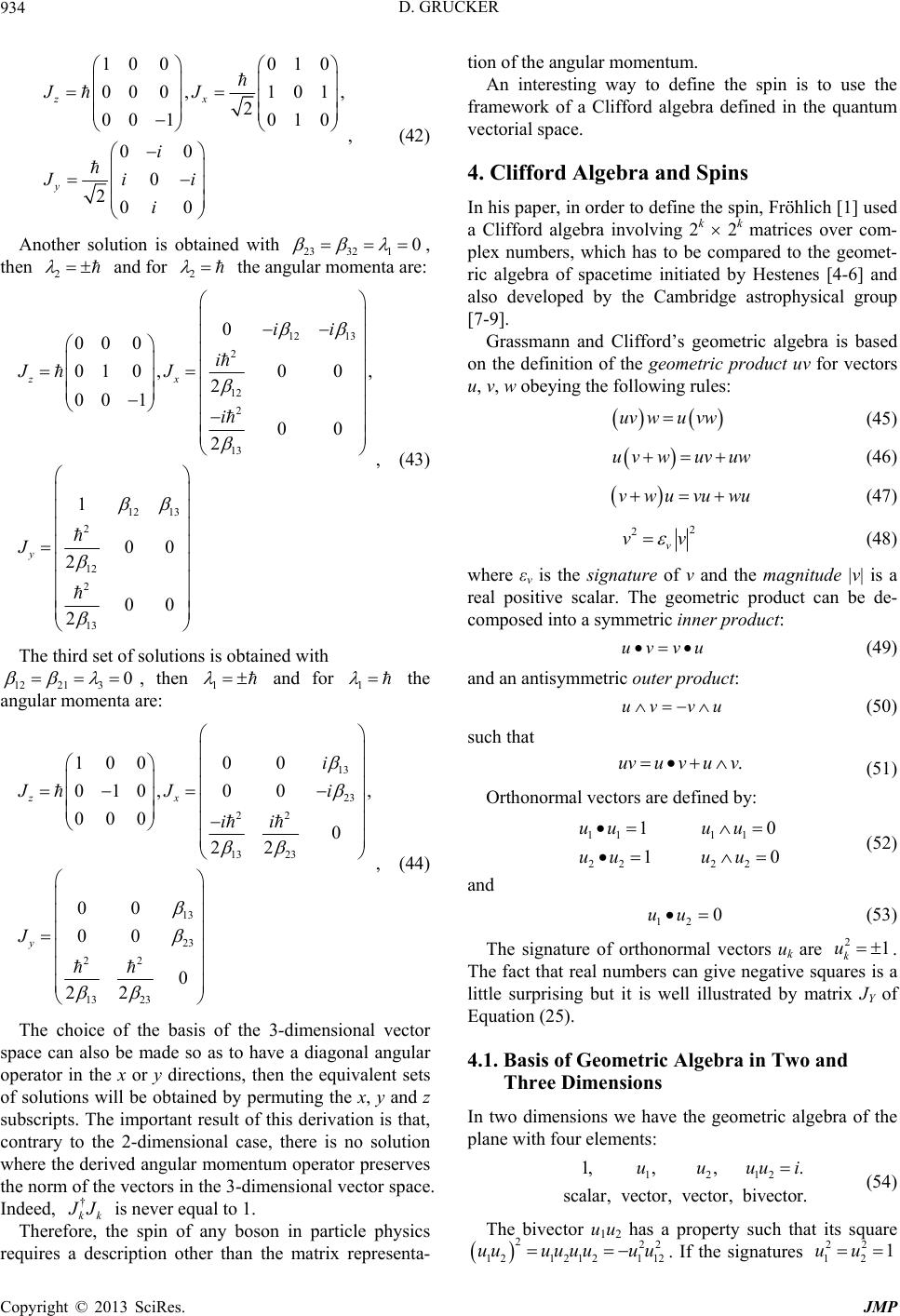 D. GRUCKER 934 10 0 00 0,2 00 1 00 0 200 zx y JJ i Jii i 010 101, 010 0 , (42) Another solution is obtained with 23321 2 , then and for 2 the angular momenta are: 12 13 00 , 00 ii 2 12 2 13 12 13 2 12 2 13 0 00 0 01 0,2 001 2 1 00 2 00 2 zx y i JJ i J , (43) The third set of solutions is obtained with 12213 0 1 , then and for 1 the angular momenta are: 13 23 22 23 0 0 , 0 i i † 13 13 23 22 13 23 100 0 010, 0 000 22 00 00 0 22 zx y JJ ii J , (44) The choice of the basis of the 3-dimensional vector space can also be made so as to have a diagonal angular operator in the x or y directions, then the equivalent sets of solutions will be obtained by permuting the x, y and z subscripts. The important result of this derivation is that, contrary to the 2-dimensional case, there is no solution where the derived angular momentum operator preserves the norm of the vectors in the 3-dimensional vector space. Indeed, kk J is never equal to 1. Therefore, the spin of any boson in particle physics requires a description other than the matrix representa- tion of the angular momentum. An interesting way to define the spin is to use the framework of a Clifford algebra defined in the quantum vectorial space. 4. Clifford Algebra and Spins In his paper, in order to define the spin, Fröhlich [1] used a Clifford algebra involving 2k 2 k matrices over com- plex numbers, which has to be compared to the geomet- ric algebra of spacetime initiated by Hestenes [4-6] and also developed by the Cambridge astrophysical group [7-9]. Grassmann and Clifford’s geometric algebra is based on the definition of the geometric product uv for vectors u, v, w obeying the following rules: uv wu vw (45) uvwuv uw (46) vwuvuwu (47) 2 2 v vv uv vu (48) where εv is the signature of v and the magnitude |v| is a real positive scalar. The geometric product can be de- composed into a symmetric inner product: uv vu (49) and an antisymmetric outer product: .uvu vuv (50) such that 111 1 222 2 10 10 uuu u uuu u (51) Orthonormal vectors are defined by: 12 0uu (52) and 21u (53) The signature of orthonormal vectors uk are k 1212 1,, ,. scalar, vector, vector, bivector. uuuui 222 1212121 12 uuuuuuu u 22 12 1uu . The fact that real numbers can give negative squares is a little surprising but it is well illustrated by matrix JY of Equation (25). 4.1. Basis of Geometric Algebra in Two and Three Dimensions In two dimensions we have the geometric algebra of the plane with four elements: (54) The bivector u1u2 has a property such that its square . If the signatures Copyright © 2013 SciRes. JMP 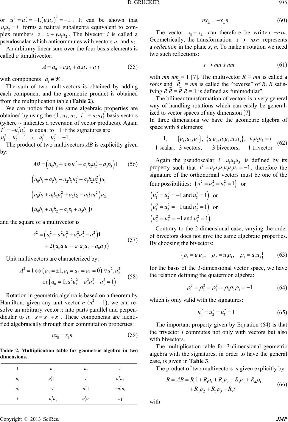 D. GRUCKER 935 or 12 . It can be shown that 12 forms a natural subalgebra equivalent to com- plex numbers 12 . The bivector i is called a pseudoscalar which anticommutes with vectors u1 and u2. 21uu zxyuu 122 3 22 121,uu uu i nxx n An arbitrary linear sum over the four basis elements is called a itmultivector: 01 aauauai a i 221 22 22 2331 (55) with components . i The sum of two multivectors is obtained by adding each component and the geometric product is obtained from the multiplication table (Table 2). We can notice that the same algebraic properties are obtained by using the {1, u1, u2, = u2u1} basis vectors (where ~ indicates a reversion of vector products). Again is equal to −1 if the signatures are or . 222 12 iuu 22 12 1uu 12 The product of two multivectors AB is explicitly given by: uu 00 111 Bababuabuab (56) 22 232 21 uabu u 01 10 23 ab abab 22 0311 2 babu u 03 1221 30 ab i 2 22 22 2 011 223 02203 1a au au a auaai 222 012312 2 2 223 11, 0, 1 02 131 2 abu a ab ab ab ab 2 A and the square of a multivector is 011 2aa u a (57) Unit multivectors are characterized by: 22 2 011 or 0, aaaa uu aua aau (58) Rotation in geometric algebra is based on a theorem by Hamilton: given any unit vector n (n2 = 1), we can re- solve an arbitrary vector x into parts parallel and perpen- dicular to n: xx nxx n u2 ui . These components are identi- fied algebraically through their commutation properties: (59) Table 2. Multiplication table for geometric algebra in two dimensions. 1 1 1 u 2 11u i 2 12 uu 2 21 uu 1 2 u i i 2 21u 2 12 uu 2 21 uu (60) The vector x can therefore be written −nxn. Geometrically, the transformation nxn represents a reflection in the plane x, n. To make a rotation we need two such reflections: mnx nm (61) with mn nm = 1 [7]. The multivector R ≡ mn is called a rotor and R = nm is called the “reverse” of R. R satis- fying R RR = 1 is defined as “unimodular”. R= The bilinear transformation of vectors is a very general way of handling rotations which can easily be general- ized to vector spaces of any dimension [7]. In three dimensions we have the geometric algebra of space with 8 elements: 123 123 123123 1, ,, ,,,, 1 scalar,1 trivector 3 vectors,3 bivectors, uuu i uuu uuuuuu (62) Again the pseudoscalar is defined by its property such that 123123 iu 12 3 iuuu 21uuuuu , therefore the signature of the orthonormal vectors must be one of the 222 123 1uuu or four possibilities: 22 2 12 3 1and1uu u or 22 2 13 2 1and1uu u or 22 2 231 1and1 .uu u Contrary to the 2-dimensional case, varying the order of bivectors does not give the same algebraic properties. By choosing the bivectors: 1122 31323 ,,uuuu uu 222 123123 1 (63) for the basis of the 3-dimensional vector space, we have the relation defining the quaternion algebra: 222 123 1uuu (64) which is only valid with the signatures: 0 11223341 52 63 7 1RABRRu RuRuR RRRi (65) The important property given by Equation (64) is that the trivector i commutes not only with vectors but also with bivectors. The multiplication table for 3-dimensional geometric algebra with the signatures, in order to have the general case, is given in Table 3. The product of two multivectors is given explicitly by: (66) with Copyright © 2013 SciRes. JMP 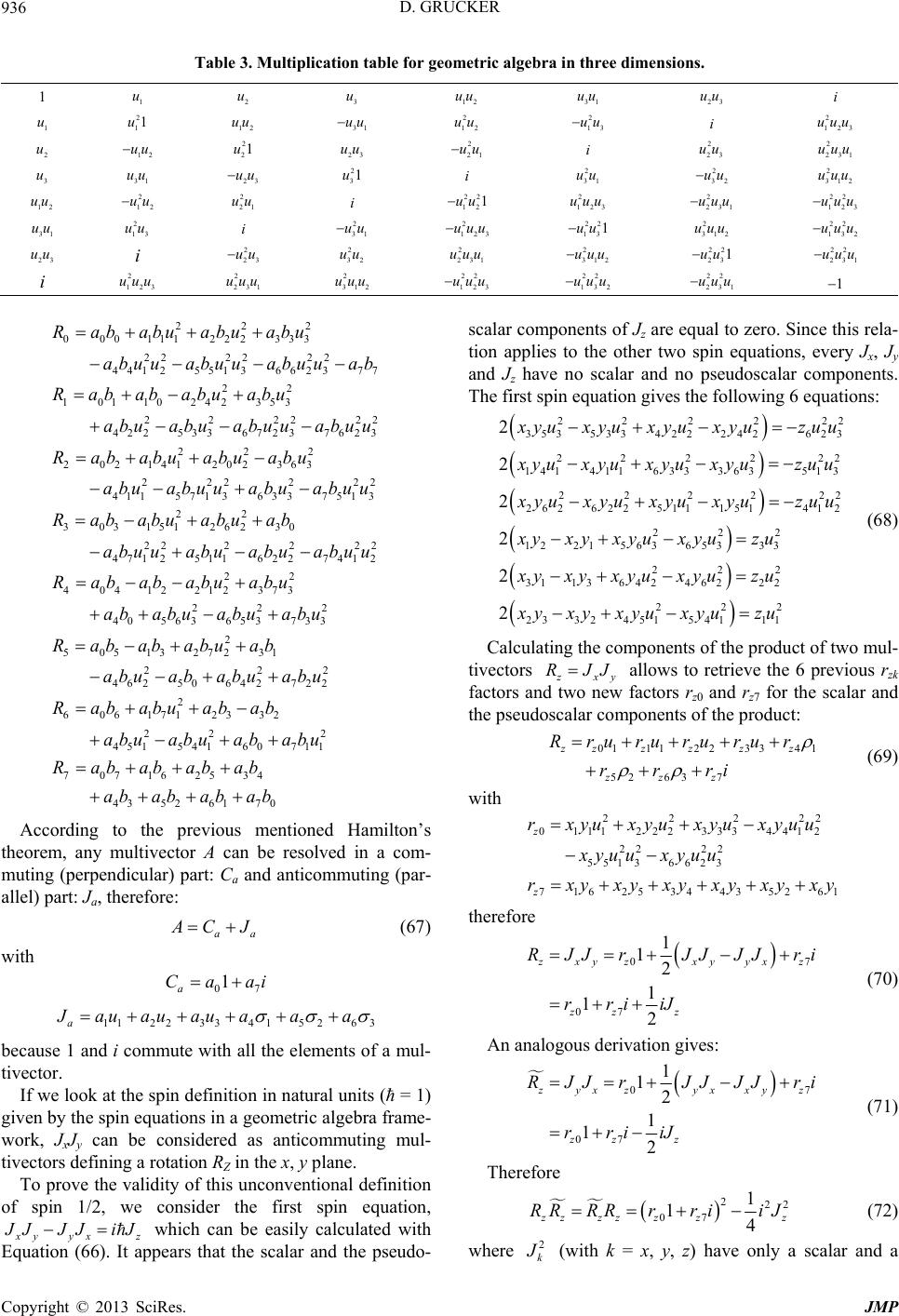 D. GRUCKER Copyright © 2013 SciRes. JMP 936 23 uu Table 3. Multiplication table for geometric algebr a in three dimensions. 1 1 u 2 u 3 u 12 uu 31 uu i 1 u u 21u1 uu 12 21u uu 31 uu uu 2 uu 12 2 uu 2 uu 13 2 123 uuu 21 2 23 uuu 2 312 uuu 21 22 123 uuu 113 22 132 uuu 3 22 231 uuu 1 i 2 3 u 12 31 uu 2 23 uu 23 2 31u i 2 uu 23 2 32 uu 1 i 2 31 uu 12 uu uu 2 uu12 2 uu 2 uu i 22 1uu 12 2 uuu 2 123 22 1uu uuu 2 uuu 23 1 2 uuu 3 2 uu i 2 uu31 2 32 uu 12 3 2 23 1 uuu 13 2 312 uuu 312 22 23 1uu i 2 23 uu i 2 uuu 12 3 2 uuu 23 1 2 uuu 312 22 uuu 12 3 22 uuu 132 22 uuu 231 222 000111222333 22 62377 22 53 22 22 3762 3 2 363 2 3 751 Rababuabuabu buuab u u abuu abu u abu 22 3 0 2 22 2 7412 22 73 2 733 1 2 722 u b u abuu u abu abu 2 2 711 abu aa 22 22 441255136 101102423 2 2 42 253367 2 22 202141202 222 41157 1363 abuuabuua Rabababuab abu abu abu Rababuabu abuabuuab 22 30315126 23 22 2 4712 51162 404122123 22 40 563653 2 505132723 22 46 25064 2 2 6061712 Ra babuabua abuuabu ab Rabababuab ab abuabu Rabababuab abuab abu Rababuab 33 22 451 541 60 707162534 43 526170 ab abu abuab Rabababab ababab ab According to the previous mentioned Hamilton’s theorem, any multivector A can be resolved in a com- muting (perpendicular) part: Ca and anticommuting (par- allel) part: Ja, therefore: CJ 07 1 a Ca ai 233415263 (67) with 11 2a aua uauaaa because 1 and i commute with all the elements of a mul- tivector. If we look at the spin definition in natural units (ħ = 1) given by the spin equations in a geometric algebra frame- work, JxJy can be considered as anticommuting mul- tivectors defining a rotation RZ in the x, y plane. To prove the validity of this unconventional definition of spin 1/2, we consider the first spin equation, yyx z JJJiJ which can be easily calculated with Equation (66). It appears that the scalar and the pseudo- scalar components of Jz are equal to zero. Since this rela- tion applies to the other two spin equations, every Jx, Jy and Jz have no scalar and no pseudoscalar components. The first spin equation gives the following 6 equations: 22 2 222 353533422242 623 22 2222 14141163336351 3 222222 262622511 151412 222 1221 56365333 222 31 1364246222 23 32 2 2 2 2 2 2 yuxyuxyuxyuzuu yu xyu xyuxyuzuu yu xyu xyu xyuzuu xyx yxyux yuzu xyxyx yux yuzu xy xy 222 451 54111 xyuxyuzu (68) Calculating the components of the product of two mul- tivectors xy RJJ allows to retrieve the 6 previous rzk factors and two new factors rz0 and rz7 for the scalar and the pseudoscalar components of the product: 011122 33 41 52 637 zzz zzz zzz R rurururur rrri 22222 0 111222333 4412 22 22 551 36623 7162534435261 z z rxyu xyu xyuxyuu xyuu xyuu r xyxyxyxyxyxy (69) with therefore 07 07 1 12 1 12 xy zxyyxz zz z RJJrJJJJ ri rriiJ (70) An analogous derivation gives: 07 07 1 12 1 12 yx zyxxyz zz z RJJrJJJJ ri rriiJ (71) Therefore 222 07 1 14 zzzz zz RRRRrriiJ 2 k (72) (with k = x, y, z) have only a scalar and a where  D. GRUCKER 937 pseudoscalar component. The important consequence is that the 2 k commute. Hamilton’s theorem proves that there exists a unit vec- tor which resolves any vector into a perpendicular and a parrallel part and u3 is a good candidate to play this role for Rz because u3 is perpendicular to any multivector Jx and any multivector Jy. The permutation of x,y,z shows that there is no incompatibility in doing so for JyJz and JzJx. We retrieve the relation (65): 222 123 1uuu (73) and find the 3 relations for 1 kk RR : 22 22 22 1 11 4 1 11 4 1 11 4 z y x i J i J i J ,, 07 07 07 zz zz yy y y xx xx RR rr RR rr RR rr (74) Therefore a spin 1/2 (S1/2) can be defined in geomet- ric algebra as a set of 3 rotors: xy yz RJJRJ x xyz JRJJ 5 26 3 3 1 (75) As Rk are unimodular vectors, they preserve the mag- nitude of multivectors. Equations (68) and (69) show that the solution for the component values of the set of the 3 rotors depends on the signatures of the orthonormal vec- tors. In summary, in geometric algebra a spin 1/2 is a set of 3 rotations obtained from the product of two multivectors which are the linear summation of 3 orthonormal vectors u, u, u and 3 bivectors , , according to: 11223 341 222 12212 ,, with k ku kukuk kxyz k k 123 (76) which fulfill the spin equations: yz JuuuJ 0JJJ 0 xy yx JJ (77) and the permutation of (x,y,z). It can be noticed that the only solution if we try to solve the spin equations in the two-dimensional case, is xyz . This result is not surprising because in two dimensions, rotations commute and . JJ 4.2. Spacetime Algebra According to Hestenes [5], the standard model for space- time is a real 4D Minkowski spacetime with vector addi- tion and scalar multiplication where we can impose the geometric product defined by equations 45 to 51 in order to generate a geometric algebra called spacetime algebra (STA). A basis for STA can be generated by a frame 1234 of orthonormal vectors which determines the pseudoscalar: ,,,uuuu 1234 iuuuu (78) In order for the pseudoscalar i to keep the same prop- erties as in the two- and three-dimensional cases, i2 must be equal to −1, which imposes two signature combina- tions which are called the metric of STA. One possibility to fulfill i2 = −1 is that three signatures should be equal to 1 and the fourth equal to −1, the second possibility is that three signatures should be equal to −1 and the fourth equal to 1. The metrics are defined by 1,1,1, 1 and 1, 1,1,1 2 2222 1 xyzt iuuuu . The 3 orthonormal vectors with identical signature will be associated with the space components x,y,z and the other with the time component t so that: 11 22 33 xyyxxt tx zx xzyt ty yzzyzt tz uuuuuu uu uuuuuu uu uuuuuuuu (79) By forming all distinct products of the four uk we ob- tain a complete basis for STA consisting of 24 = 16 line- arly independent elements. There are 12 bivectors obtained from the arrangement of 2 out of the 4 orthonormal vectors, but there are only 6 with different magnitudes: (80) As regards trivectors, there are 24 products to be ob- tained from the arrangement of 3 out of the 4 orthonor- mal vectors. There are 8 distinct products and only four- having different magnitudes: 0 2 1 2 2 2 3 2 t xyzxzy t x ytz yzt x y xt zx zt y z xt yx yt z iu uuuuuuu iu uuuuuu u iu uuu uuuu iu uuuuuu u (81) 1234 1scalar :1 4vectors :,,, 6trivectors :3,3 4pseudovectors: 1 pseudoscalar: uuuu i We can verify that i anticommutes with vectors and trivectors but commutes with bivectors. A complete basis for STA is: (82) Copyright © 2013 SciRes. JMP  D. GRUCKER 938 According to the 3-dimensional geometric algebra case we have the quaternion relation (64) for the bivectors. By adequately choosing the bivectors of the vector space basis, the 3 new bivectors σk fulfill the fol- lowing quaternion relation: 2 22 1231 iiii 23 1ii 2 3 3 1 t t u u 1,1,1, 1 (83) The four pseudovectors are: ξ0 the pseudoscalar of di- mension 3 and the three other ξk which, again, fulfill a quaternion relation between the geometric product of the time orthonormal vector and ξk: 22 12 12 tt tt uu uu (84) The 3 quaternion relations are verified with the metric and the choice of the basis defined by Equa- tions (80) and (81). For the other metric, Equation (84) is still valid, but to keep the quaternion relations (63) and (83) for bivectors, we have to consider another basis where 22 z, which corresponds to reverse rotations in the x,z plane. uu 1 2 3 ,,, If we consider the geometric algebra definition of spin 1/2 given by Equations (76) to (77) we retrieve the spin 1/2 characterized by the 6-element multivector: ,,,1 ,, yzx y Suu z z u (85) but in the 4-dimensional vector space there are two other spins 1/2: ,,,21 2 2222 ,, ,i ,i,i ,,, , xyzxyz xyzzty Suuu uuu uuuu 3 22 123 , t xt uu (86) ,,,3,,, ,,, xyzx y z xyzt Suuu uuuu 1 23 222 123 , , , , t tt t t uuu u u 1,1,1, 1 (87) for the metric . For the other metric with the other basis there are three new spins 1/2 obtained from the 3 vectors ux, uy and uz: 1 2 3 ,,, z u ,,,4 ,, xyzx y Suu (88) 22 22 ,,,5 1 ,,, , xyzxyzzty t Su u uuuuu22 2 3 ,xt uu 2 2 3 , , t t uu (89) 22 ,,,6 1 ,,, xyzx yz t Suuuu ,,,1..6,, ,1..6 ,, ztyzt SSS 444 444444 1122 33 4451 62738192 103 110 12 1132143 ,, with ,, (90) There are 18 other spins 1/2 obtained with the different vectors of the 4-dimensional case and the same bivectors: ,,,1..6xyt x (91) Therefore the 24 spins 1/2 found with the matrix deri- vation are retrieved in the STA description but here with a clear distinction between spins 1/2 which fall in two metric-dependent categories. If the 12 spins 1/2 of each category were sorted as a function of bivectors we would find 3 families of 4 spins 1/2 as in elementary particle physics. As the definition of rotation given by Equation (61) applies whatever the dimension of the vector space, in four dimensions the spin 1 can be defined by set of 3 rotors: xyyzyx yz k RJJ RJJ RJJ Jkukukukuk kkkkk k kkk kxyz 2221uuu (92) where the Jk fulfill the spin equations. From the gener- alization to 4 dimensions of the vector product given by Equation (66), it is easy to see that the scalar component is null because real components commute and the pseudo scalar component is null because its parts are independ- ent of the signatures. As the Rk are unimodular vectors, they induce rotations which preserve the norm of any vector. Again the solution to the equations which deter- mine the components of the multivectors Jk is dependent on the signature of the orthonormal vectors. Therefore there are 4 different solutions with space-like signatures xyz 21u and time-like signature t and 12 different solutions if we consider each signature in- dependently. 5. Conclusion We have shown that for the two-dimensional complex vector space, the spin matrices can be calculated directly from the angular momentum commutator definition. We have retrieved the 3 Pauli matrices and found 23 other triplet solutions. When extended to the three-dimensional space, we have shown that there is no matrix which pre- serves the norm of the vectors and fulfills the spin equa- tions. By using a geometric algebra with a vector prod- uct which combines a commuting product and an anti- commuting product it has been possible in four-dimen- sional spacetime to retrieve the 24 different spins 1/2 defined as 12 clockwise and 12 counter-clockwise rota- tions. These rotations are characterized by anticommut- ing parts composed of 3 vectors and 3 bivectors which fulfill the spin equations. Spin 1 can be defined as 3 rota- tions characterized by 4 vectors, 6 bivectors and 4 trivectors which fulfill the spin equations. These uni- modular spin 1 rotations preserve the magnitude of mul- tivectors. There are 12 different spins 1 depending on the signature of the 4 orthonormal vectors of the four-di- mensional vector space. The correspondence between this derivation and particle physics is perhaps fortuitous but the use of STA offers the advantage of formulating Copyright © 2013 SciRes. JMP  D. GRUCKER Copyright © 2013 SciRes. JMP 939 conventional relativistic physics in invariant form with- out reference to a coordinate system [5] and it seems promising to analyze how time evolution and spin inter- action can be used in order to predict the gyromagnetic ratio of the proton and the neutron. 6. Acknowledgements I would like to thank Jacques Baudon, Edward Belaga, Jules Grucker, Tarek Khalil, Jean Richert, Kees van Schenk Brill for enlightening, and Nathalie Heider for liberating my mind. REFERENCES [1] J. Fröhlich, “Spin or Actually: Spin and Quantum Statis- tics p1-60 in The Spin, Poincaré Seminar 2007,” B. Du- plantier, J. M. Raimond and V. Rivasseau, Eds., Birk- häuser, Basel, 2009. [2] C. Cohen-Tannoudji, B. Diu and F. Laloë, “Quantum Me- chanics,” Wiley, New York, 1977. [3] P. A. M. Dirac, “The Principles of Quantum Mechanics,” Oxford University Press, Oxford, 1930, pp. 157-162,281- 285. [4] D. Hestenes, American Journal of Physics, Vol. 47, 1979, p. 399. doi:10.1119/1.11806 [5] D. Hestenes, American Journal of Physics, Vol. 71, 2003, pp. 691-714. doi:10.1119/1.1571836 [6] D. Hestenes, American Journal of Physics, Vol. 71, 2003, pp. 104-121. doi:10.1119/1.1522700 [7] S. Gull, A. Lasenby and C. Doran, Foundations of Phys- ics, Vol. 23, 1993, pp. 1175-1201. doi:10.1007/BF01883676 [8] C. Doran, A. Lasenby and S. Gull, Foundations of Phys- ics, Vol. 23, 1993, pp. 1239-1264. doi:10.1007/BF01883678 [9] J. Lasenby, A. N. Lasenby and C. J. L. Doran, Philoso- phical Transactions of the Royal Society A, Vol. 358, 2000, pp. 21-39. doi:10.1098/rsta.2000.0517
|