Enhancing the Performance of Ultra-Tight Integration of GPS/PL/INS: A Federated Filter Approach

Paper Menu >>

Journal Menu >>

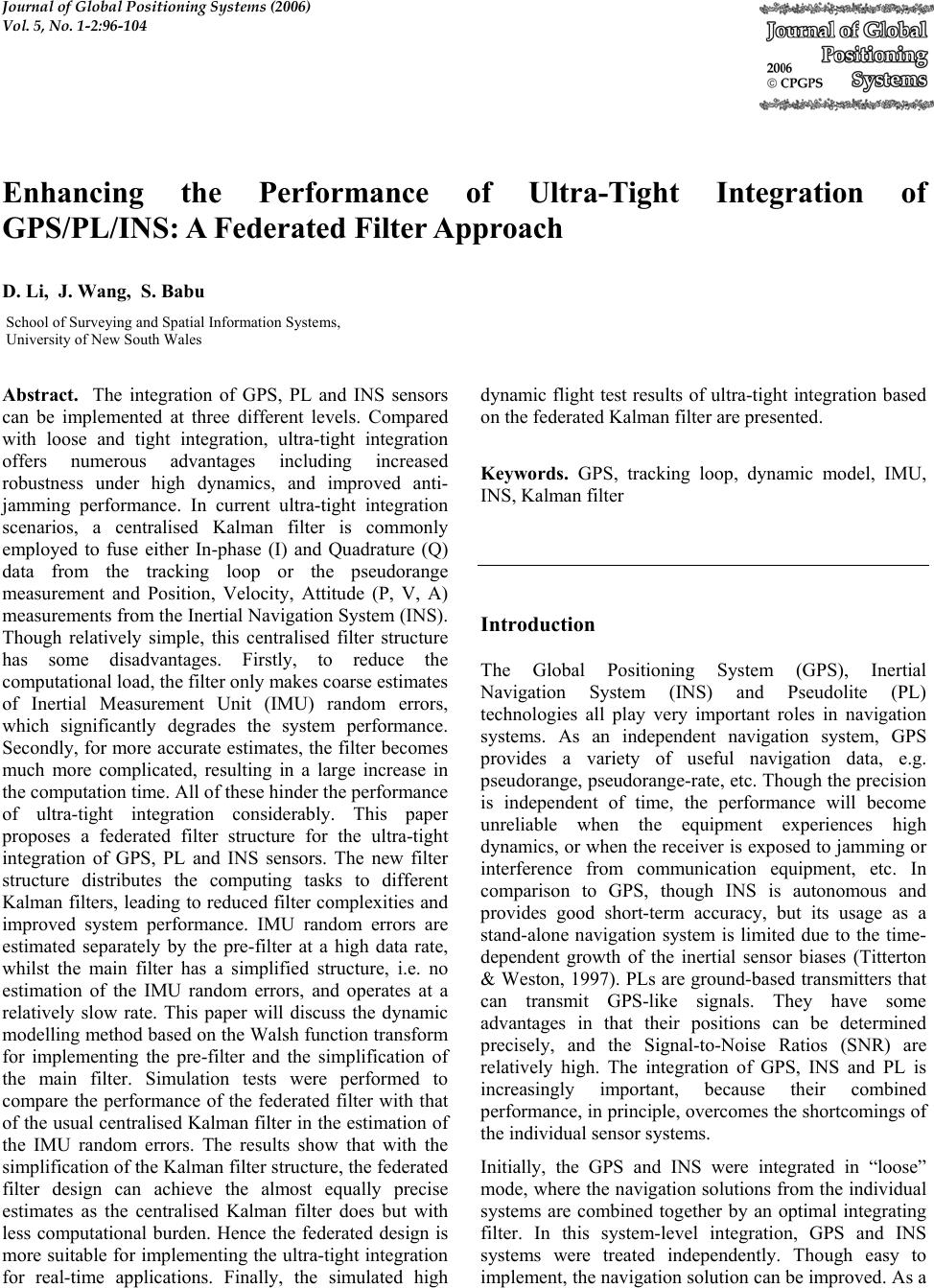Journal of Global Positioning Systems (2006)

Vol. 5, No. 1-2:96-104

Enhancing the Performance of Ultra-Tight Integration of

GPS/PL/INS: A Federated Filter Approach

D. Li, J. Wang, S. Babu

School of Surveying and Spatial Information Systems,

University of New South Wales

Abstract. The integration of GPS, PL and INS sensors

can be implemented at three different levels. Compared

with loose and tight integration, ultra-tight integration

offers numerous advantages including increased

robustness under high dynamics, and improved anti-

jamming performance. In current ultra-tight integration

scenarios, a centralised Kalman filter is commonly

employed to fuse either In-phase (I) and Quadrature (Q)

data from the tracking loop or the pseudorange

measurement and Position, Velocity, Attitude (P, V, A)

measurements from the Inertial Navigation System (INS).

Though relatively simple, this centralised filter structure

has some disadvantages. Firstly, to reduce the

computational load, the filter only makes coarse estimates

of Inertial Measurement Unit (IMU) random errors,

which significantly degrades the system performance.

Secondly, for more accurate estimates, the filter becomes

much more complicated, resulting in a large increase in

the computation time. All of these hinder the performance

of ultra-tight integration considerably. This paper

proposes a federated filter structure for the ultra-tight

integration of GPS, PL and INS sensors. The new filter

structure distributes the computing tasks to different

Kalman filters, leading to reduced filter complexities and

improved system performance. IMU random errors are

estimated separately by the pre-filter at a high data rate,

whilst the main filter has a simplified structure, i.e. no

estimation of the IMU random errors, and operates at a

relatively slow rate. This paper will discuss the dynamic

modelling method based on the Walsh function transform

for implementing the pre-filter and the simplification of

the main filter. Simulation tests were performed to

compare the performance of the federated filter with that

of the usual centralised Kalman filter in the estimation of

the IMU random errors. The results show that with the

simplification of the Kalman filter structure, the federated

filter design can achieve the almost equally precise

estimates as the centralised Kalman filter does but with

less computational burden. Hence the federated design is

more suitable for implementing the ultra-tight integration

for real-time applications. Finally, the simulated high

dynamic flight test results of ultra-tight integration based

on the federated Kalman filter are presented.

Keywords. GPS, tracking loop, dynamic model, IMU,

INS, Kalman filter

Introduction

The Global Positioning System (GPS), Inertial

Navigation System (INS) and Pseudolite (PL)

technologies all play very important roles in navigation

systems. As an independent navigation system, GPS

provides a variety of useful navigation data, e.g.

pseudorange, pseudorange-rate, etc. Though the precision

is independent of time, the performance will become

unreliable when the equipment experiences high

dynamics, or when the receiver is exposed to jamming or

interference from communication equipment, etc. In

comparison to GPS, though INS is autonomous and

provides good short-term accuracy, but its usage as a

stand-alone navigation system is limited due to the time-

dependent growth of the inertial sensor biases (Titterton

& Weston, 1997). PLs are ground-based transmitters that

can transmit GPS-like signals. They have some

advantages in that their positions can be determined

precisely, and the Signal-to-Noise Ratios (SNR) are

relatively high. The integration of GPS, INS and PL is

increasingly important, because their combined

performance, in principle, overcomes the shortcomings of

the individual sensor systems.

Initially, the GPS and INS were integrated in “loose”

mode, where the navigation solutions from the individual

systems are combined together by an optimal integrating

filter. In this system-level integration, GPS and INS

systems were treated independently. Though easy to

implement, the navigation solution can be improved. As a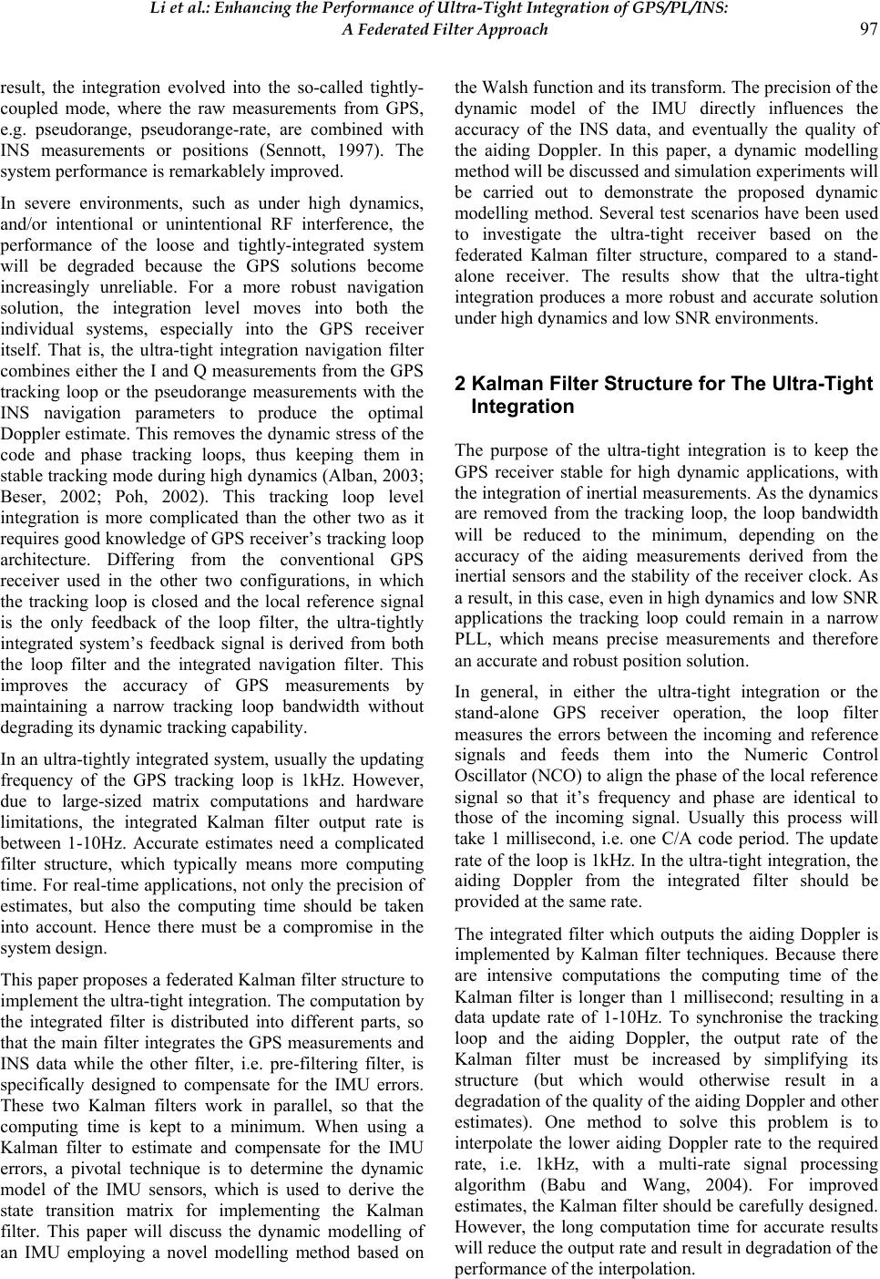

Li et al.: Enhancing the Performance of Ultra-Tight Integration of GPS/PL/INS:

A Federated Filter Approach 97

result, the integration evolved into the so-called tightly-

coupled mode, where the raw measurements from GPS,

e.g. pseudorange, pseudorange-rate, are combined with

INS measurements or positions (Sennott, 1997). The

system performance is remarkablely improved.

In severe environments, such as under high dynamics,

and/or intentional or unintentional RF interference, the

performance of the loose and tightly-integrated system

will be degraded because the GPS solutions become

increasingly unreliable. For a more robust navigation

solution, the integration level moves into both the

individual systems, especially into the GPS receiver

itself. That is, the ultra-tight integration navigation filter

combines either the I and Q measurements from the GPS

tracking loop or the pseudorange measurements with the

INS navigation parameters to produce the optimal

Doppler estimate. This removes the dynamic stress of the

code and phase tracking loops, thus keeping them in

stable tracking mode during high dynamics (Alban, 2003;

Beser, 2002; Poh, 2002). This tracking loop level

integration is more complicated than the other two as it

requires good knowledge of GPS receiver’s tracking loop

architecture. Differing from the conventional GPS

receiver used in the other two configurations, in which

the tracking loop is closed and the local reference signal

is the only feedback of the loop filter, the ultra-tightly

integrated system’s feedback signal is derived from both

the loop filter and the integrated navigation filter. This

improves the accuracy of GPS measurements by

maintaining a narrow tracking loop bandwidth without

degrading its dynamic tracking capability.

In an ultra-tightly integrated system, usually the updating

frequency of the GPS tracking loop is 1kHz. However,

due to large-sized matrix computations and hardware

limitations, the integrated Kalman filter output rate is

between 1-10Hz. Accurate estimates need a complicated

filter structure, which typically means more computing

time. For real-time applications, not only the precision of

estimates, but also the computing time should be taken

into account. Hence there must be a compromise in the

system design.

This paper proposes a federated Kalman filter structure to

implement the ultra-tight integration. The computation by

the integrated filter is distributed into different parts, so

that the main filter integrates the GPS measurements and

INS data while the other filter, i.e. pre-filtering filter, is

specifically designed to compensate for the IMU errors.

These two Kalman filters work in parallel, so that the

computing time is kept to a minimum. When using a

Kalman filter to estimate and compensate for the IMU

errors, a pivotal technique is to determine the dynamic

model of the IMU sensors, which is used to derive the

state transition matrix for implementing the Kalman

filter. This paper will discuss the dynamic modelling of

an IMU employing a novel modelling method based on

the Walsh function and its transform. The precision of the

dynamic model of the IMU directly influences the

accuracy of the INS data, and eventually the quality of

the aiding Doppler. In this paper, a dynamic modelling

method will be discussed and simulation experiments will

be carried out to demonstrate the proposed dynamic

modelling method. Several test scenarios have been used

to investigate the ultra-tight receiver based on the

federated Kalman filter structure, compared to a stand-

alone receiver. The results show that the ultra-tight

integration produces a more robust and accurate solution

under high dynamics and low SNR environments.

2 Kalman Filter Structure for The Ultra-Tight

Integration

The purpose of the ultra-tight integration is to keep the

GPS receiver stable for high dynamic applications, with

the integration of inertial measurements. As the dynamics

are removed from the tracking loop, the loop bandwidth

will be reduced to the minimum, depending on the

accuracy of the aiding measurements derived from the

inertial sensors and the stability of the receiver clock. As

a result, in this case, even in high dynamics and low SNR

applications the tracking loop could remain in a narrow

PLL, which means precise measurements and therefore

an accurate and robust position solution.

In general, in either the ultra-tight integration or the

stand-alone GPS receiver operation, the loop filter

measures the errors between the incoming and reference

signals and feeds them into the Numeric Control

Oscillator (NCO) to align the phase of the local reference

signal so that it’s frequency and phase are identical to

those of the incoming signal. Usually this process will

take 1 millisecond, i.e. one C/A code period. The update

rate of the loop is 1kHz. In the ultra-tight integration, the

aiding Doppler from the integrated filter should be

provided at the same rate.

The integrated filter which outputs the aiding Doppler is

implemented by Kalman filter techniques. Because there

are intensive computations the computing time of the

Kalman filter is longer than 1 millisecond; resulting in a

data update rate of 1-10Hz. To synchronise the tracking

loop and the aiding Doppler, the output rate of the

Kalman filter must be increased by simplifying its

structure (but which would otherwise result in a

degradation of the quality of the aiding Doppler and other

estimates). One method to solve this problem is to

interpolate the lower aiding Doppler rate to the required

rate, i.e. 1kHz, with a multi-rate signal processing

algorithm (Babu and Wang, 2004). For improved

estimates, the Kalman filter should be carefully designed.

However, the long computation time for accurate results

will reduce the output rate and result in degradation of the

performance of the interpolation.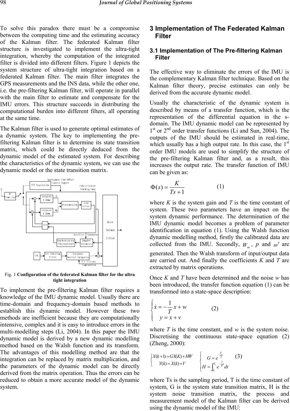

98 Journal of Global Positioning Systems

To solve this paradox there must be a compromise

between the computing time and the estimating accuracy

of the Kalman filter. The federated Kalman filter

structure is investigated to implement the ultra-tight

integration, whereby the computation of the integrated

filter is divided into different filters. Figure 1 depicts the

system structure of ultra-tight integration based on a

federated Kalman filter. The main filter integrates the

GPS measurements and the INS data, while the other one,

i.e. the pre-filtering Kalman filter, will operate in parallel

with the main filter to estimate and compensate for the

IMU errors. This structure succeeds in distributing the

computational burden into different filters, all operating

at the same time.

The Kalman filter is used to generate optimal estimates of

a dynamic system. The key to implementing the pre-

filtering Kalman filter is to determine its state transition

matrix, which could be directly deduced from the

dynamic model of the estimated system. For describing

the characteristics of the dynamic system, we can use the

dynamic model or the state transition matrix.

Fig. 1 Configuration of the federated Kalman filter for the ultra

tight integration

To implement the pre-filtering Kalman filter requires a

knowledge of the IMU dynamic model. Usually there are

time-domain and frequency-domain based methods to

establish this dynamic model. However these two

methods are inefficient because they are computationally

intensive, complex and it is easy to introduce errors in the

multi-modelling steps (Li, 2004). In this paper the IMU

dynamic model is derived by a new dynamic modelling

method based on the Walsh function and its transform.

The advantages of this modelling method are that the

integration can be replaced by matrix multiplication, and

the parameters of the dynamic model can be directly

derived from the matrix operation. Thus the errors can be

reduced to obtain a more accurate model of the dynamic

system.

3 Implementation of The Federated Kalman

Filter

3.1 Implementation of The Pre-filtering Kalman

Filter

The effective way to eliminate the errors of the IMU is

the complementary Kalman filter technique. Based on the

Kalman filter theory, precise estimates can only be

derived from the accurate dynamic model.

Usually the characteristic of the dynamic system is

described by means of a transfer function, which is the

representation of the differential equation in the s-

domain. The IMU dynamic model can be represented by

1st or 2nd order transfer functions (Li and Sun, 2004). The

outputs of the IMU should be estimated in real-time,

which usually has a high output rate. In this case, the 1st

order IMU models are used to simplify the structure of

the pre-filtering Kalman filter and, as a result, this

increases the output rate. The transfer function of IMU

can be given as:

)( +

=Φ Ts

s (1)

where K is the system gain and T is the time constant of

system. These two parameters have an impact on the

system dynamic performance. The determination of the

IMU dynamic model becomes a problem of parameter

identification in equation (1). Using the Walsh function

dynamic modelling method, firstly the calibrated data are

collected from the IMU. Secondly, m

W, p and T

are

generated. Then the Walsh transform of input/output data

are carried out. And finally the coefficients K and T are

extracted by matrix operations.

Once K and T have been determined and the noise w has

been introduced, the transfer function equation (1) can be

transformed into a state-space description:

⎪

⎩

⎪

⎨

⎧

+−=

vxy

& (2)

where T is the time constant, and w is the system noise.

Discretising the continuous state-space equation (2)

(Zheng, 2000):

⎩

⎨

⎧

+=+

VkXkY

WHKGXkX

)()(

)()1(

⎪

⎩

⎪

⎨

⎧

∫−

−

dteH

(3)

where Ts is the sampling period, T is the time constant of

system, G is the system state transition matrix, H is the

system noise transition matrix, the process and

measurement model of the Kalman filter can be derived

using the dynamic model of the IMU: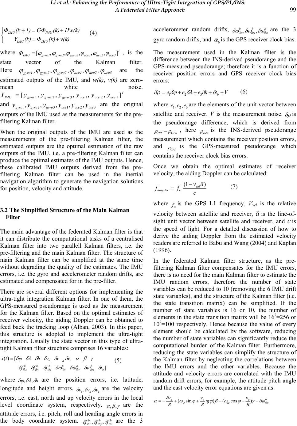

Li et al.: Enhancing the Performance of Ultra-Tight Integration of GPS/PL/INS:

A Federated Filter Approach 99

⎩

⎨

⎧

+=+

v(k)(k)Φ(k)Y

Hw(k)(k)GΦ1)(kΦ

IMUIMU

IMUIMU (4)

where T

acc3acc2acc1gyro2gyro2gyro1IMU

Φ],,,,,[

ϕϕϕϕϕϕ

=, is the

state vector of the Kalman filter.

Here acc3acc2acc1gyro2gyro2gyro1

,,,,, are the

estimated outputs of the IMU, and w(k), v(k) are zero-

mean white noise.

accaccaccgyrogyrogyroIMU yyyyyyY ],,,,,[ 321321

and 321321 ,,,,, accaccaccgyrogyrogyro yyyyyy are the original

outputs of the IMU used as the measurements for the pre-

filtering Kalman filter.

When the original outputs of the IMU are used as the

measurements of the pre-filtering Kalman filter, the

estimated outputs are the optimal estimation of the raw

outputs of the IMU, i.e. a pre-filtering Kalman filter can

produce the optimal estimates of the IMU outputs. Hence,

these calibrated IMU outputs derived from the pre-

filtering Kalman filter can be used in the inertial

navigation algorithm to generate the navigation solutions

for position, velocity and attitude.

3.2 The Simplified Structure of the Main Kalman

Filter

The main advantage of the federated Kalman filter is that

it can distribute the computational tasks of a centralised

Kalman filter into two parallell Kalman filters, i.e. the

pre-filtering and the main Kalman filter. The structure of

main Kalman filter can be simplified at the same time

without degrading the quality of the estimates. The IMU

errors, i.e. the gyro and accelerometer random drifts, are

estimated and compensated for in the pre-filter.

There are several different options for implementing the

ultra-tight integration Kalman filter. In one of them, the

GPS-measured pseudorange is used as the measurement

for the Kalman filter. Based on the optimal estimates of

receiver velocity, the aiding Doppler can be obtained to

feed back the tracking loop (Alban, 2003). In this paper,

this structure is adopted to implement the ultra-tight

integration. Usually the state vector in this type of ultra-

tight Kalman filter structure comprises 16 variables:

]

[)(

ibz

iby

ibx

ibz

iby

ibx

tfff

vvvhtx

δδωδωδωδδδ

δλ

δϕ

=(5)

where h

δλ

δϕ

,,are the position errors, i.e. latitude,

longitude and height errors. zne vvv

δδδ

,, are the velocity

errors, i.e. east, north and up velocity errors in the local

level coordinate system, respectively.

,, are the

attitude errors, i.e. pitch, roll and heading angle errors in

the body coordinate system. b

ibz

iby

ibx fff

δδδ

,, are the 3

accelerometer random drifts, b

ibz

iby

ibx

δωδωδω

,, are the 3

gyro random drifts, and b

is the GPS receiver clock bias.

The measurement used in the Kalman filter is the

difference between the INS-derived pseudorange and the

GPS-measured pseudorange; therefore it is a function of

receiver position errors and GPS receiver clock bias

errors:

Vtheee b

δλ

δϕ

321 (6)

where 321 ,, eee are the elements of the unit vector between

satellite and receiver. V is the measurement noise.

δρ

the pseudorange difference, which is derived from

GPSINS

ρρ

−, here INS

is the INS-derived pseudorange

measurement which contains the receiver position errors,

and GPS

is the GPS-measured pseudorange which

contains the receiver clock bias errors.

Once we obtain the optimal estimates of receiver

velocity, the aiding Doppler can be calculated:

ff vel

txdoppler

)1(

−

= (7)

where tx

fis the GPS L1 frequency, Vvel is the relative

velocity between satellite and receiver, a

ris the line-of-

sight unit vector between satellite and receiver, and cis

the speed of light. For a detailed discussion of how to

derive the aiding Doppler from the estimated velocity

readers are referred to Babu and Wang (2004) and Kaplan

(1996).

In the federated Kalman filter structure, as the pre-

filtering Kalman filter compensates for the IMU errors,

there is no need for the main Kalman filter to estimate the

IMU random errors, therefore the number of state

variables can be reduced to 10 (removing the 6 IMU drift

state variables), and the structure of the Kalman filter (i.e.

the state transition matrix) can be simplified. If the

number of state variables is 16 or 10, the number of

elements in the state transition matrix will be 162=256 or

102=100 respectively. Hence because the value of every

element should be calculated by the software, reducing

the number of state variables can significantly reduce the

computational burden of the Kalman filter. Furthermore,

reducing the state variables can simplify the structure of

the Kalman filter by neglecting the correlations between

the IMU errors and the other variables. Because the

attitude and velocity errors are correlated with the IMU

random drift errors, for example, the attitude pitch angle

and the east velocity error equations are given as:

ibx

δωγϕωβϕϕω

−+−++−=)cos()sin(

100 Journal of Global Positioning Systems

ibyxzn

vtg

fffv

δδδϕϕϕω

δδϕωδγαδ

−−+−

+−+−=

)seccos2(

)sin(2

& (8)

where hRR e+=, e

Rand h is the earth radius and height

respectively, and ie

is the angle rate of earth rotation.

zx ff,are the accelerometer measurements in the body

coordinate system.

In the federated Kalman filter structure, the pre-filtering

Kalman filter estimates and compensates for the IMU

random drifts, thus the main Kalman filter doesn’t need

to estimate them. As described above, the correlations of

the IMU random drift errors with the other state variables

can be neglected. The attitude and velocity error equation

could be simplified:

γϕωβϕϕω

)cos()sin(

n+−++−=

iexzn

vtg

ffv

δδδϕϕϕω

δδϕωγαδ

−−+−

+−−=

)seccos2(

)sin(2

& (9)

Hence the state transition matrix can be simplified. Here

we still use the pseudorange differences as the

measurements for the Kalman filter. Hence the

measurement model is the same as that in the centralised

Kalman filter, which is described by equation (6).

4 Experimental Results

4.1 IMU Dynamic Modelling Results

Given the 2nd order dynamic system:

153.0

)( 2

=ssasas

bsb

sG (10)

the Walsh function modelling results are shown in Table

1. Using these modelling results the dynamic models are

constructed, as shown in Figure 2. The dashed lines

represent the outputs of these models and the solid lines

represent the outputs of the model in equation (10) which

were applied to the same unit step input signal.

Table 1. Modeling results of method using different numbers of Walsh

function

Model

Parameters 1

a 2

a 1

b 2

0.53 1 0 1

8 Walsh

function 0.92627 1.9058 -1.1183 1.9138

32 Walsh

function 0.54293 1.0162 -0.16551 1.0163

128 Walsh

function 0.53035 1.0009 -

0.0054747 1.001

256 Walsh

function 0.53018 1.0002 -0.020797 1.0002

The results show that the accuracy of the estimated model

parameters depends on the number of Walsh functions

used for the modelling. For the simulation test, 128

Walsh functions produce good modelling results.

4.2 Pre-filtering Kalman Filter Testing Results

First, the flight trajectory with known dynamics, with

characteristics shown in Table 2, was generated.

Fig. 2 Modeling results of different number of Walsh function

A comparison between IMU outputs with/without using

the pre-filtering Kalman filter was made in order to study

how the pre-filtering improves the IMU outputs. In the

simulation test, the dynamics of the trajectory are known,

i.e. the position, attitude and velocity, and the original

IMU outputs could be deduced from this information.

After adding noise to the original IMU outputs, the

simulated raw IMU outputs corresponding to the flight

trajectory could be obtained. Simulation time lasts for 60

sec. The output rate of the IMU is 100Hz. Figure 3

depicts the IMU outputs that have large errors from the

known trajectory.

Table 2. Parameters of flight trajectory

Initial position

(latitude, longitude,

high) (degree)

45° 45° 0

Initial velocity

(east, north, up) (m/s) 1 1 0

Initial acceleration

(m/s2)

0 0 0

Initial attitude

(roll, pitch, heading)

(degree)

0 0 45°

Simulation time(s) 60

Simulation time step (s) 0.01

Flight status Constant acceleration = 0.5g

After optimally estimating the IMU outputs by the pre-

filtering Kalman filter, most of the IMU random drift

errors were removed, and the filtered IMU outputs are

Li et al.: Enhancing the Performance of Ultra-Tight Integration of GPS/PL/INS:

A Federated Filter Approach 101

shown in Figure 4, indicating an improvement in IMU

outputs.

4.3 Main Kalman Filter Testing Results

To test the performance of the federated Kalman filter,

the comparison of the estimates from these two

configurations, i.e. the federated and centralised Kalman

filter, is carried out.

Fig. 3 Original outputs of IMU

In the centralised Kalman filter structure, the IMU

random drifts errors are estimated together with other

state variables. The optimal navigation solutions of

position, attitude and velocity, represented as the latitude,

longitude, earth-level velocity and roll, pitch, heading

(compensated by the estimated errors derived from the

Kalman filter) are shown in Figure 5.

In the federated Kalman filter, as the IMU random drift

errors are already estimated during the pre-filtering, the

main Kalman filter doesn’t need to estimate the IMU

errors again. To compare with the results of the

centralised Kalman filter, the compensated position,

attitude and velocity are given in Figure 6. From Figure 6

it can be observed that the federated Kalman filter

delivers the same precision of estimates as the centralised

Kalman filter approach, however the computing time is

greatly reduced because of the simplified state transition

matrix. Hence, the update rate of the estimates can be

increased, which is helpful when implementing the

Kalman filter for real-time applications.

4.4 Ultra-Tight GPS/INS Receiver Experimental

Results

As shown in the previous section, the federated Kalman

filter structure velocity estimates with the same accuracy

as the centralised Kalman filter.

Fig. 4 Filtered outputs of IMU

102 Journal of Global Positioning Systems

Fig. 5 Navigation solutions based on the centralised Kalman filter

structure

Therefore the accuracies of the aiding Doppler for both

configurations is of the same level, which means that the

ultra-tight GPS/INS receiver based on the federated

Kalman receiver has the same quality of output as the

centralised Kalman filter, but benefits from faster

compution.

Figure 7 illustrates the performance of the ultra-tightly

integrated GPS/INS receiver and the stand-alone GPS

receiver. The tracking loop bandwidth is set at 12Hz.

Normally, by comparing the power of the carrier tracking

loop with the tracking threshold it can be determined if

the tracking loop is in FLL or PLL mode, which

illustrates the stability and accuracy of the tracking loop.

As mentioned above, the FLL means lower

measurements accuracy. For better tracking effect, the

tracking mode should quickly switch from FLL to PLL.

From Figure 7 it can be shown that when the dynamics of

the simulated trajectory is high, the stand-alone GPS

receiver tracking loop had large tracking errors and

remained in the FLL mode. Once the dynamics become

larger or the bandwidth is reduced, it will lose lock.

However, the ultra-tightly integrated receiver could

remain in the PLL tracking mode with the same

dynamics, therefore it can be concluded that the ultra-

tight integrated receiver is more robust for the high

dynamic applications.

Usually the variety of the code loop power represents the

stability of the code tracking loop. If it is large enough to

exceed the threshold, the code tracking loop will lose

lock. Because the carrier tracking loop relies on the

stability of the code tracking loop, it will also lose lock at

the same time. Figure 8 shows that the variety of code

loop power of the ultra-tight receiver is smaller than that

of a stand-alone receiver, meaning it has more stable

tracking capability.

The Q measurements represent the tracking loop errors.

Figure 9 demonstrates that the ultra-tight receiver has

smaller tracking errors than the stand-alone receiver

under the same dynamic conditions, i.e. more accurate

measurements could be obtained from the tracking loop.

Fig. 6 Navigation solutions based on the federated Kalman filter

structure

Li et al.: Enhancing the Performance of Ultra-Tight Integration of GPS/PL/INS:

A Federated Filter Approach 103

Fig. 7 Comparison of tracking loop status between the ultra tight

integration and stand-alone receiver

5 Concluding Remarks

In this paper a federated Kalman filter structure for the

ultra-tight integration of GPS/INS/PL has been

investigated, in which the IMU random errors are

estimated and compensated for by a pre-filtering Kalman

filter. In this way the computational burden can be

separated into different parts and processed in parallel.

The pivotal technique to implement this structure, the

dynamic modelling method of the IMU based on the

Walsh function and its transform, is investigated and the

simulation experiments have demonstrated its accuracy

and feasibility. The Kalman filter was implemented on

the IMU dynamic model. Test results have shown that the

IMU errors can be effectively removed by pre-filtering so

that the accuracy of the aiding Doppler derived from the

integrated Kalman filter is the same as that of the

centralised Kalman filter, but requires less computation

time. This federated Kalman filter structure is therefore

especially attractive, especially for real-time applications.

Fig. 8 Code tracking loop status

Fig. 9 Tracking loop Q measurements

Acknowledgments

This research is supported by an ARC (Australian

Research Council) – Discovery Research Project on

‘Robust Positioning Based on Ultra-tight Integration of

GPS, Pseudolites and Inertial Sensors’. The authors

would like to thank Prof. Chris Rizos for his valuable

comments on the early version of this paper.

References

Li D., Sun Y. (2004) Research of The Dynamic Modelling of

FOG Based on Walsh Function. Ship Engineering, Dec,

2004

Alban S., Akos D., Rock S. & Gebre-Egziobher D. (2003)

Performance Analysis and Architectures for INS-Aided

GPS tracking loops. Institute of Navigation – NTM,

Anaheim, CA, 22-24 January, 611-622.

Kaplan E.D. (1996) Understanding GPS: Principles and

Applications. Artech House, MA. 119-207

Tsui J.B.Y. (2000) Fundamentals of Global Positioning

Receivers – A Software Approach. John Wiley & Sons,

Inc. 165-190

Beser J., Alexander S., Crane R., Rounds S., Wyman J., Baeder

B. (2002) TrunavTM: A Low-Cost Guidance/Navigation

Unit Integrating a SAASM-based GPS and MEMS IMU

in a Deeply Coupled Mechanization. 15th Int. Tech.

Meeting of the Satellite Division of the U.S. Inst. of

Navigation, Portland, OR, 24-27 September, 545-555.

Babu R., Wang J. (2004) Comparative study of interpolation

techniques for ultra-tight integration of GPS/INS/PL

sensors. GNSS 2004, Sydney, Australia, 6-8 Dec.

Babu R., Wang J. (2004) Improving the Quality of IMU-

Derived Doppler Estimates for Ultra-Tight GPS/INS

Integration. GNSS 2004, Rotterdam, The Netherlands, 16-

19 May.

Farrell J.A. & Barth M. (1999) The Global Positioning System

and Inertial Navigation. McGraw-Hill.

104 Journal of Global Positioning Systems

Hentschel T. & Fettweis G. (2000) Sample Rate Conversion for

Software Radio. IEEE Communications Magazine,

August, 2-10.

Mitra S.K. (1999) Digital Signal Processing – A Computer

Based Approach. Tata McGraw-Hill Edition, India, ISBN

0-07-463723-1.

Vaidyanathan P.P. (1990) Multirate Digital Filter, Filter

Banks, Polyphase Networks, and Applications: A

Tutorial. Proc. IEEE, 78, 56-93.

Wang J., Dai L., Tsuiji T., Rizos C., Grejner-Brzezinska D.,

Toth C. (2001) GPS/INS/Pseudolite Integration:

Concepts, Simulation and Testing. 14th Int. Tech.

Meeting of the Satellite Division of the U.S. Inst. of

Navigation, Salt Lake City, Ohio, 11-14 September, 2708-

2715.

Ward P. (1998) Performance Comparisons Between FLL, PLL

and a Novel FLL-Assisted PLL Carrier Tracking Loop

Under RF Interference Conditions. 11th Int. Tech.

Meeting of the Satellite Division of the U.S. Inst. of

Navigation, Nashville, Tennessee, 15-18 September, 783-

795.