Journal of Transportation Technologies, 2013, 3, 204-213
http://dx.doi.org/10.4236/jtts.2013.33021 Published Online July 2013 (http://www.scirp.org/journal/jtts)
Contribution to the Investigation of Motorcyclists’ Speed
Prediction Equations for Two-Lane Rural Roads
Panagiotis V. Lemonakis1, Nikolaos E. Eliou1, George N. Botzoris2, Theodoros E. Karakasidis1
1Department of Civil Engineering, Section of Transportation, University of Thessaly, Volos, Greece
2Department of Civil Engineering, Section of Transportation, Democritus Thrace University, Xanthi, Greece
Received March 21, 2013; revised April 22, 2013; accepted April 30, 2013
Copyright © 2013 Panagiotis V. Lemonakis et al. This is an open access article distributed under the Creative Commons Attribution
License, which permits unrestricted use, distribution, and reproduction in any medium, provided the original work is properly cited.
ABSTRACT
The calculation of speed prediction equations has been the subject of numerous researches in the past. The majority of
them present models to predict free-flow speed in terms of the road geometry at the curved road sections and more spe-
cifically in terms of the radiuses of the curves. Common characteristic is that none of them approaches the speed be-
havior of motorcycles since they are excluded from the datasets of the various studies. Instead, the models usually pre-
dict operating speed for other vehicle types such as passenger cars, vans, pickups and trucks. The present paper aims to
cover this gap by developing speed prediction equations for motorcycles. For this purpose a new methodology is pro-
posed while field measurements were carried out in order to obtain an adequate dataset of free-flow speeds along the
curved sections of three different two lane rural roads. The aforementioned field measurements were conducted by two
participants incorporating various road conditions (e.g. light conditions, experience level, familiarity with the routes).
The ultimate target was the development of speed prediction equations by calculating the optimum regression curves
between the curve radius’ and the corresponding velocities for the different road conditions. The research revealed that
the proposed methodology could be used as a very useful tool to investigate motorcyclists’ behavior at curved road sec-
tions. Moreover it was feasible to draw conclusions correlating the speed adjustment with the various driving condi-
tions.
Keywords: Motorcyclists’ Behavior; Regression Curves; Curvature; Free-Flow Speed; Speed Equations; Field
Measurements
1. Introduction
Numerous studies have been carried out during the last
decades in the field of road safety in order to predict the
relationship between driver behavior and road features
(especially on horizontal curves). Many of these studies
focus on creating analytical models expressing driver
behavior in relation to the characteristics of the roads
[1-7]. In these models, driver behavior is expressed by
the operating speed (V85, that represents the 85th-percen-
tile speed), while the road characteristics are generally
represented by the curvature change rate of the single
curve or the horizontal curve radius, since it has been
estimated that the magnitude of the radius of the hori-
zontal curves is the most considerable factor that deter-
mines operational speed [8]. Nevertheless, the true effect
of each individual geometric variable (e.g. curve radius,
length of the curve, deflection angle and superelevation)
is still not known precisely in quantitative terms [9].
As stated in a recent study [10], most models devel-
oped to date focus on passenger car speeds. However, the
speed behavior of motorcycles was studied by [11],
evaluated the possibility to develop a motorcycle operat-
ing speed prediction model analyzing the relationships
between the motorcycle operating speed and the passen-
ger cars operating speed. Both motorcycle and vehicle
speeds were collected using a Light Detection and Rang-
ing (Lidar) gun while graphic as well as statistical analy-
sis followed the measurements. The outcome of this re-
search was the development of the Equation (1):
2
85 85
1.162, 0.94 
PTW PC
VVR (1)
where
V85PTW: the 85th percentile speed on tangent of power-
two-wheelers (km/h),
V85PC: the 85th percentile speed on tangent of passen-
ger cars (km/h),
R2: the coefficient of determination.
C
opyright © 2013 SciRes. JTTs

P. V. LEMONAKIS ET AL. 205
The objective in another study by [12] is to develop a
speed prediction equation on horizontal curves using the
geometric characteristics of the curves at 11 sites in ex-
clusive motorcycle lane. To achieve this objective, the
speeds of motorcyclists were measured in exclusive mo-
torcycle lanes in Malaysia using two devices; a portable
laser speed detector and a digital video camera. The au-
thors of this study using linear regression procedure, in
order to identify the best fit combinations of the inde-
pendent variables, developed the following Equation (2):
85,curve 19.3570.394 0.654VWT (2)
where
V85,curve: the 85th percentile motorcycle speed on hori-
zontal curves,
W: the total lane width,
Δ: deflection angle,
T: the length of tangent.
No other study relevant to motorcycle speed prediction
equations has been carried out apart from the two
afore-mentioned ones, at least to our knowledge. There-
fore the impact of the different light conditions, the dif-
ferent experience level, the familiarity with the road and
the different road environment to drivers’ behavior ex-
pressed in operating speed changes can only be observed
in passenger cars studies.
The investigation of motorcyclists’ speed prediction
equations at the present study has been achieved by pro-
posing a new methodology of measuring speeds based on
GPS technology which preceded the conduction of field
measurements in order to in order to obtain an adequate
dataset of free-flow speeds. The field measurements were
designed taking into account various factors that poten-
tially influence the riders’ behavior such as the different
light conditions, the difference on the riding experience
level, the familiarity of the riders with the routes, the
presence of pillion and the different road environments,
such as width/condition of the road pavement, roadside
land use, etc.
2. Experimental Design of the Field
Measurements
2.1. Participants
Initially, three basic parameters had to be defined with
regards to the participants’ selection that would execute
the field measurements; demographic criteria, riding ex-
perience and psychometric aspects of the riders [13].
The choice of the participants’ gender was based on
preceding researches which have shown that males are
over-represented both in car and motorcycle accidents
[14,15], but also in the riding population even though
they do not necessarily demonstrate riskier behaviors.
Moreover, males constitute the typical rider gender and
they can be recruited easier than the female ones.
Experience is also a significant factor that determines
the level of risk taking behavior among riders. In most of
the cases, there is a correlation between riding experience
and age, since young riders are more inexperienced in
comparison to the older ones who are more experienced.
In order to reduce the probability of accident occurrence
during the experiment, young and older riders were ex-
cluded, due to their high risk rates. Consequently, all
participants had to have an actual riding experience of at
least 5 years and should not be older than 50 years old.
Aiming also to the latter target, the sample of riders was
biased towards riders with limited accident records. Fur-
thermore, since one of the main objectives of the present
research was to determine how the riding experience
affects riding behavior, efforts were made in order to
match the overall participants’ features apart from their
riding experience, which was selected to be considerably
different.
Another issue that had to be dealt with was that the
riders had to achieve a certain level of familiarity with
the instrumented motorcycle. For that reason, prior to the
execution of the field measurements, the riders were
asked to ride the experimental motorcycle until they felt
confident with its operation. It should also be noted that
the demands for adequate handling were relatively in-
creased due to the size and weight of the instrumented
motorcycle.
Taking under consideration the afore-mentioned, two
male riders belonging at the same age group were se-
lected to carry out the field measurements. None of them
revealed any obvious reason of impaired riding ability
while their riding experience levels were totally different.
Moreover, they had common stay of residence, adjacent
to the routes where the experiment was conducted and
therefore, they both had similar familiarity with the ex-
perimental environment.
2.2. Instrumented Vehicle and Record Devices
Many researchers have obtained speed data, using in
most cases, a radar gun [16,17] as well as speed detectors
[12]. Both methods can introduce errors such as measur-
ing errors or can influence drivers’ behavior who might
perceive the speed record equipment and hence, adjust
their speeds to the legal speed limits of the sections stud-
ied [10]. Therefore in order to overcome the shortcom-
ings of the speed recording equipment that has been used
so far we established a new speed record method which
was based on the usage of GPS data logger.
Data loggers can record GPS, video and vehicle data
and are ideally suited to motorsport due to their small
weight, size and increased accuracy. Moreover without
fitting any other sensors, the measure of speed, track po-

P. V. LEMONAKIS ET AL. 206
sition, distance, lap time, lateral acceleration, longitudi-
nal acceleration and height is feasible. Recording of such
parameters can be particularly useful especially in cases
where driving behavior is not approached exclusively in
speed terms. In addition, by using a single record system
it is possible to investigate the behavior of the riders in
multiple curves, since the various equipment are attached
onto the vehicle instead of the road.
In this view the equipment that was used to record the
relevant with the riding performance parameters, such as
position and velocity was the Video Vbox from Race-
logic Company. The Video Vbox combines a powerful
GPS data logger with a high quality solid-state video
recorder. In order to capture the video file, it is equipped
with two cameras and two microphones whilst records
the following parameters as standard along with the
video file: satellites, time, latitude, longitude, velocity,
heading, height and vertical velocity.
The videos, as well as the data files are saved onto an
SD card. The logging rate is ten samples per second,
which was considered as adequate enough to cover the
needs of the experiment. As an example, an 8-gigabyte
high capacity SD card, logging video on the highest
quality setting was able to log approximately 160 min-
utes of video. Apparently, this is an approximation, as
the size of the recorded video depended on what was
being recorded. The motion, color and complexity of the
subject matter affected the size of the video file created.
It should also be mentioned that the size of the data file
was particularly small, in comparison to the size of the
video file. The recorded data were downloaded daily
right after the execution of the experiment from the flash
memory to an external High Capacity HD that was given
to the riders.
The primary specifications of the record device are
summarized in Table 1 and the accuracies of the re-
corded quantities are indicated in Table 2.
Lastly, the instrumented bike that was used to carry
out the field measurements was an on/off motorcycle,
widespread on rural roads especially because of its abil-
ity to provide sufficient transport on asphalt, as well as
on soil material surfaces. The primary specifications of
the instrumented motorcycle are summarized in Table 3.
2.3. Location, Type of Roads, Weather
Conditions, Time of Day
The selection of the experimental environment had to be
based upon four primary conditions: the location, the
type of the road, the weather conditions and finally, the
time and date that the experiment would be conducted.
All of these four conditions had to be common for both
riders in order to record comparable data.
The location of the experiment should ensure on one
hand the constant function of the recording device, and
Table 1. Specifications of equipment video vbox.
Video file MPEG-4
Recording
options
- Record only when moving (default),
- Continuous record,
- Record start/stop via optional remote switch.
Camera
inputs 2 × AV camera inputs (camera supplied as option)
with integrated 12V power supplies
Graphics 24 bit color - DVD 720 × 576 at 25 frames/sec or
DVD 720  480 at 30 frames/sec resolution options
Sound - 2 × external microphone connections,
- MP2 (MPEG1 Layer II) encoded video stream.
Storage
options SD Card
Table 2. Accuracies of equipment video vbox.
Parameter Accuracy
Velocity ±0.2 Km/h
Distance ±0.05%
Position ±5 m
Height ±10 m
Lateral acceleration ±0.5%
Longitudinal acceleration ±0.5%
Table 3. Specifications of the instrumented motorcycle.
Category Enduro/offroad
Displacement 652.00 ccm
Engine type Single cylinder, 4-stroke
Power 48.00 HP
Torque 57.00 Nm
Top speed 160.0 km/h
0 - 100 km/h 5.20 seconds
60 to 140 km/h, highest gear 10.60 seconds
Cooling system Liquid
Gearbox 5-speed
Transmission type Chain
Front suspension travel 170 mm
Rear suspension travel 165 mm
Front tire dimensions 100/90 - 19
Rear tire dimensions 130/80 - 17
Front/rear brakes Single disc
Brakes diameter Front: 300 mm, Rear: 240 mm
Weight incl. oil, gas, etc. 199.0 kg
Seat height 820 mm
Fuel capacity 17.50 liters
Starter Electric

P. V. LEMONAKIS ET AL. 207
on the other hand the presence of a large number of
curved sections. Moreover, the traffic volumes should be
particularly limited during the experiment in order to
achieve unaffected riding behavior. Finally, for purely
practical purposes, the experimental environment was
sought close to the participants’ place of residence. Tak-
ing into account the above-mentioned, the road network
that would serve the needs of the research and meet the
requirements of the experiment was mountain Pelion, in
Magnesia, Central Greece. The road network of Pelion
consists exclusively of intensive curved rural roads,
which vary depending on its geometrical characteristics,
the presence of vertical/horizontal signage and the pave-
ment condition.
In a more detailed investigation, three road sections
were determined as appropriate to carry out the field
measurements (Figure 1). The evaluation of the appro-
priate experimental road sections is indicated in Table 4.
Regarding the weather conditions and in order to re-
strict the parameters that affect the riding behavior of the
participants, both riders instructed to cease the measure-
ments when the pavement was wet, even slightly. The
natural lighting level should be constant and hence, dur-
ing cloudy or foggy days the measurements were ceased
as well. In general, the instructions that were given to the
riders, forbidden the execution of the experiment in case
any environmental or traffic conditions might divert their
regular riding behavior. It is also noted that the unim-
peded approach to the curves ensured by succeeding null
traffic volumes. For that purpose the measurements were
conducted when the road was free from the presence of
other road users.
Aiming at the investigation of the correlation between
natural lighting and riding behavior, two different time
periods were set for the execution of the experiment. The
first one was set between 09:00 and 16:00 (constant natu-
ral lighting during autumn-daytime measurements) and
the second one between 21:00 and 01:00 (nighttime
measurements). Apparently, apart from the lighting con-
ditions all the other environmental and weather condi-
tions were equivalent for both time periods.
Apart from the investigation of the correlation between
lighting conditions and riding behavior, another aim of
the present research was the inquiry of the contribution
of the familiarity with a road to the riding behavior. For
that purpose the participants were asked to ride each one
of the routes six times during daytime and six times dur-
ing nighttime. Finally, after the completion of the twelve
afore-mentioned measurements, the riders were asked to
repeat each route once more with the presence of a pil-
lion in order to investigate how this condition influences
their riding behavior since the presence of a pillion af-
fects firstly the total weight of the system rider/motorcy-
cle and secondly it increases the sense of responsibility
of the rider for the pillion’s safety. In total, both riders
conducted 78 measurements, as analytically shown in
Table 5.
3. Data Analysis
The data analysis was based on three program packages;
Vbox Tools v2.2.2 b042 of Racelogic, Excel 2007 of
Microsoft and Autocad 2009 of Autodesk. The original
data files recorded at the SD card (extension *.vbo)
opened using Vbox Tools and then were simply con-
verted to comma delimited files (extension *.csv). Each
*.csv file corresponded to a specific measurement and
contained 3 columns; velocity, coordinate x and coordi-
nate y. It is reminded that these values were recorded at a
sampling rate of 10 Hz.
Table 4. Evaluation of the experimental routes.
Road section
(coordinates)
Afyssos-Afeta i
(39˚16'30.24"Β,
23˚10'1.12"Α to
39˚16'53.69"Β,
23˚10'41.10"Α)
Milina-Lafkos
(39˚10'6.58"Β,
23˚13'43.97"Α to
39˚10'0.43"Β,
23˚14'21.94"Α)
Neohori-
Kalama ki
(39˚18'43.98"Β,
23˚12'49.28"Αto
39˚19'23.41"Β
23˚11'45.51"Α)
Length 2300 m 2300 m 2550 m
Curve radius
range
(Rmin /Rmax )11 m/315 m 24 m/157 m 49 m/222 m
Total
pavement
width
5.20 m (2.60 m
per direction)
6.00 m (3.00
per direction)
8.20 m (4.10 m
per direction)
Horizontal
signage Absent
Continuous single
line on the
centerline as well
as on the
boundaries of the
road
Yes
Vertical
signage Absent Partially
(3 danger signs) Yes
Guard railsAbsent Absent Yes
Artificial
lighting Absent Absent Absent
Pavement
condition
Extensive
surfaces with
cracks, grooves
and subsidence
Several spots with
transverse and
longitudinal
cracks, grooves
and layering of
bituminous seal
Excellent
Evaluation Poor Satisfactory Excellent
Table 5. Amount and description of measur eme nts.
Condition Number
of routesNumber of repetitions Number of ridersTotal
Daytime 3 6 2 36
Nighttime 3 6 2 36
Pillion 3 1 2 6
Total amount of measurements 78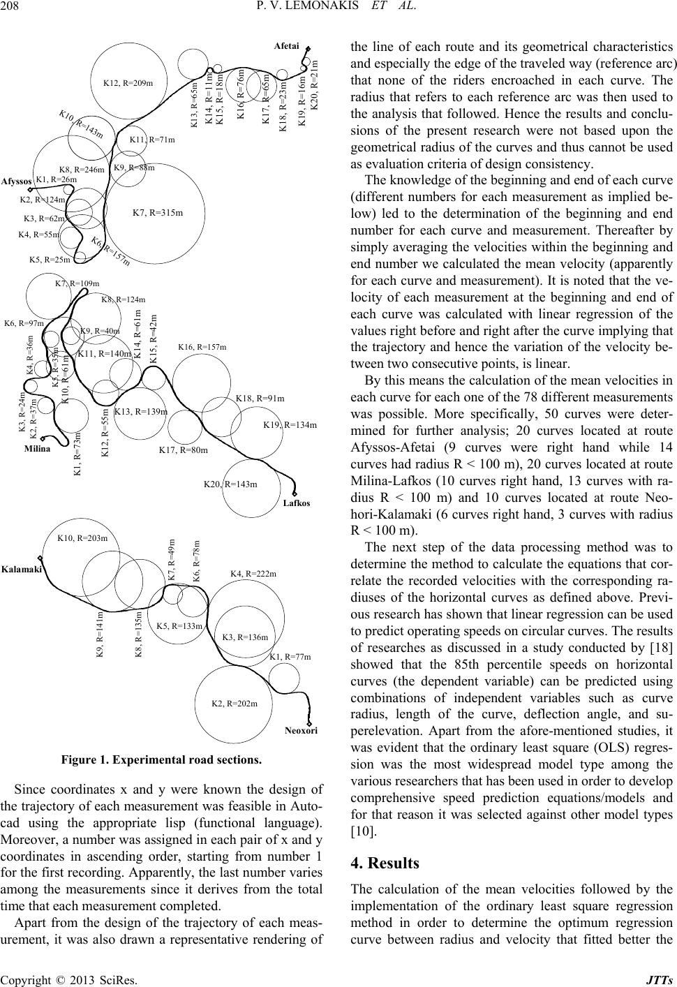

P. V. LEMONAKIS ET AL. 208
K14, R=11m
K20, R=21m
K19, R=16m
K15, R=18m
K16, R=76m
K17, R=65m
K18, R=23m
K7, R=315m
K1, R=26m
K2, R=124m
K3, R=62m
K8, R=246m
K10, R=143m
K13, R=65m
K4, R=55m
K5, R=25m
K6, R=157m
K12, R=209m
K11, R=71m
K9, R=88m
Afyssos
Afetai
K1, R=73m
K2, R=37m
K3, R=24m
K4, R=36m
K9, R=40m
K15, R=42m
K16, R=157m
K17, R=80m
K18, R=91m
K19, R=134m
K20, R=143m
K14, R=61m
K13, R=139m
K12, R=55m
K11, R=140m
K5, R=35m
K6, R=97m
K7, R=109m
K8, R=124m
K10, R=61m
Lafkos
Milina
K1, R=77m
K2, R=202m
K3, R=136m
K4, R=222m
K10, R=203m
K9, R=141m K8, R=135m
K7, R=49m
K6, R=78m
K5, R=133m
Neoxori
Kalamaki
Figure 1. Experimental road sections.
Since coordinates x and y were known the design of
the trajectory of each measurement was feasible in Auto-
cad using the appropriate lisp (functional language).
Moreover, a number was assigned in each pair of x and y
coordinates in ascending order, starting from number 1
for the first recording. Apparently, the last number varies
among the measurements since it derives from the total
time that each measurement completed.
Apart from the design of the trajectory of each meas-
urement, it was also drawn a representative rendering of
the line of each route and its geometrical characteristics
and especially the edge of the traveled way (reference arc)
that none of the riders encroached in each curve. The
radius that refers to each reference arc was then used to
the analysis that followed. Hence the results and conclu-
sions of the present research were not based upon the
geometrical radius of the curves and thus cannot be used
as evaluation criteria of design consistency.
The knowledge of the beginning and end of each curve
(different numbers for each measurement as implied be-
low) led to the determination of the beginning and end
number for each curve and measurement. Thereafter by
simply averaging the velocities within the beginning and
end number we calculated the mean velocity (apparently
for each curve and measurement). It is noted that the ve-
locity of each measurement at the beginning and end of
each curve was calculated with linear regression of the
values right before and right after the curve implying that
the trajectory and hence the variation of the velocity be-
tween two consecutive points, is linear.
By this means the calculation of the mean velocities in
each curve for each one of the 78 different measurements
was possible. More specifically, 50 curves were deter-
mined for further analysis; 20 curves located at route
Afyssos-Afetai (9 curves were right hand while 14
curves had radius R < 100 m), 20 curves located at route
Milina-Lafkos (10 curves right hand, 13 curves with ra-
dius R < 100 m) and 10 curves located at route Neo-
hori-Kalamaki (6 curves right hand, 3 curves with radius
R < 100 m).
The next step of the data processing method was to
determine the method to calculate the equations that cor-
relate the recorded velocities with the corresponding ra-
diuses of the horizontal curves as defined above. Previ-
ous research has shown that linear regression can be used
to predict operating speeds on circular curves. The results
of researches as discussed in a study conducted by [18]
showed that the 85th percentile speeds on horizontal
curves (the dependent variable) can be predicted using
combinations of independent variables such as curve
radius, length of the curve, deflection angle, and su-
perelevation. Apart from the afore-mentioned studies, it
was evident that the ordinary least square (OLS) regres-
sion was the most widespread model type among the
various researchers that has been used in order to develop
comprehensive speed prediction equations/models and
for that reason it was selected against other model types
[10].
4. Results
The calculation of the mean velocities followed by the
implementation of the ordinary least square regression
method in order to determine the optimum regression
curve between radius and velocity that fitted better the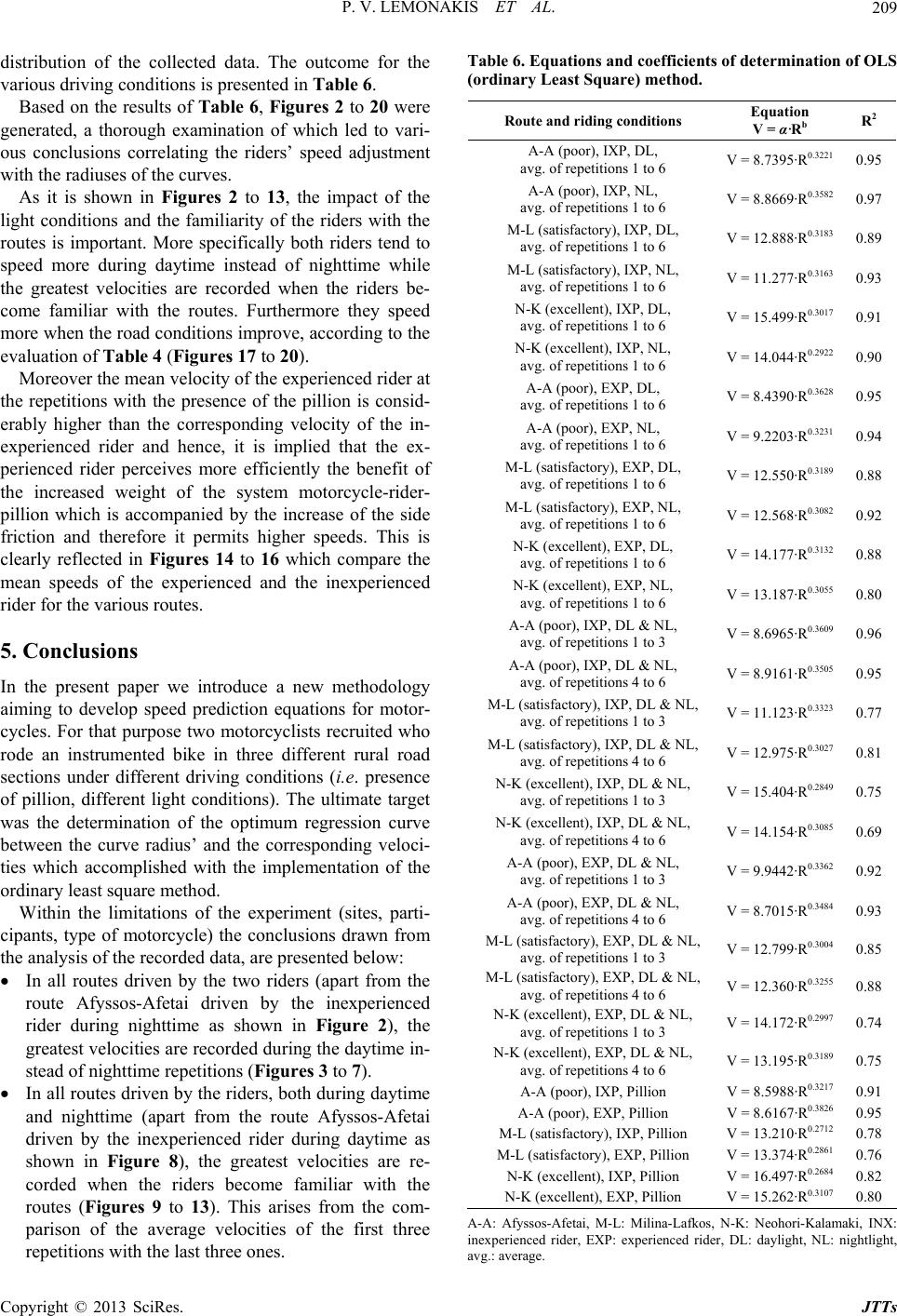

P. V. LEMONAKIS ET AL. 209
distribution of the collected data. The outcome for the
various driving conditions is presented in Table 6.
Based on the results of Table 6, Figures 2 to 20 were
generated, a thorough examination of which led to vari-
ous conclusions correlating the riders’ speed adjustment
with the radiuses of the curves.
As it is shown in Figures 2 to 13, the impact of the
light conditions and the familiarity of the riders with the
routes is important. More specifically both riders tend to
speed more during daytime instead of nighttime while
the greatest velocities are recorded when the riders be-
come familiar with the routes. Furthermore they speed
more when the road conditions improve, according to the
evaluation of Table 4 (Figures 17 to 20).
Moreover the mean velocity of the experienced rider at
the repetitions with the presence of the pillion is consid-
erably higher than the corresponding velocity of the in-
experienced rider and hence, it is implied that the ex-
perienced rider perceives more efficiently the benefit of
the increased weight of the system motorcycle-rider-
pillion which is accompanied by the increase of the side
friction and therefore it permits higher speeds. This is
clearly reflected in Figures 14 to 16 which compare the
mean speeds of the experienced and the inexperienced
rider for the various routes.
5. Conclusions
In the present paper we introduce a new methodology
aiming to develop speed prediction equations for motor-
cycles. For that purpose two motorcyclists recruited who
rode an instrumented bike in three different rural road
sections under different driving conditions (i.e. presence
of pillion, different light conditions). The ultimate target
was the determination of the optimum regression curve
between the curve radius’ and the corresponding veloci-
ties which accomplished with the implementation of the
ordinary least square method.
Within the limitations of the experiment (sites, parti-
cipants, type of motorcycle) the conclusions drawn from
the analysis of the recorded data, are presented below:
 In all routes driven by the two riders (apart from the
route Afyssos-Afetai driven by the inexperienced
rider during nighttime as shown in Figure 2), the
greatest velocities are recorded during the daytime in-
stead of nighttime repetitions (Figures 3 to 7).
 In all routes driven by the riders, both during daytime
and nighttime (apart from the route Afyssos-Afetai
driven by the inexperienced rider during daytime as
shown in Figure 8), the greatest velocities are re-
corded when the riders become familiar with the
routes (Figures 9 to 13). This arises from the com-
parison of the average velocities of the first three
repetitions with the last three ones.
Table 6. Equations and coefficients of de te r mination of OLS
(ordinary Least Square) method.
Route and riding conditions Equation
V = α·Rb R2
A-A (poor), IXP, DL,
avg. of repetitions 1 to 6 V = 8.7395·R0.3221 0.95
A-A (poor), IXP, NL,
avg. of repetitions 1 to 6 V = 8.8669·R0.3582 0.97
M-L (satisfactory), IXP, DL,
avg. of repetitions 1 to 6 V = 12.888·R0.3183 0.89
M-L (satisfactory), IXP, NL,
avg. of repetitions 1 to 6 V = 11.277·R0.3163 0.93
N-K (excellent), IXP, DL,
avg. of repetitions 1 to 6 V = 15.499·R0.3017 0.91
N-K (excellent), IXP, NL,
avg. of repetitions 1 to 6 V = 14.044·R0.2922 0.90
A-A (poor), EXP, DL,
avg. of repetitions 1 to 6 V = 8.4390·R0.3628 0.95
A-A (poor), EXP, NL,
avg. of repetitions 1 to 6 V = 9.2203·R0.3231 0.94
M-L (satisfactory), EXP, DL,
avg. of repetitions 1 to 6 V = 12.550·R0.3189 0.88
M-L (satisfactory), EXP, NL,
avg. of repetitions 1 to 6 V = 12.568·R0.3082 0.92
N-K (excellent), EXP, DL,
avg. of repetitions 1 to 6 V = 14.177·R0.3132 0.88
N-K (excellent), EXP, NL,
avg. of repetitions 1 to 6 V = 13.187·R0.3055 0.80
A-A (poor), IXP, DL & NL,
avg. of repetitions 1 to 3 V = 8.6965·R0.3609 0.96
A-A (poor), IXP, DL & NL,
avg. of repetitions 4 to 6 V = 8.9161·R0.3505 0.95
M-L (satisfactory), IXP, DL & NL,
avg. of repetitions 1 to 3 V = 11.123·R0.3323 0.77
M-L (satisfactory), IXP, DL & NL,
avg. of repetitions 4 to 6 V = 12.975·R0.3027 0.81
N-K (excellent), IXP, DL & NL,
avg. of repetitions 1 to 3 V = 15.404·R0.2849 0.75
N-K (excellent), IXP, DL & NL,
avg. of repetitions 4 to 6 V = 14.154·R0.3085 0.69
A-A (poor), EXP, DL & NL,
avg. of repetitions 1 to 3 V = 9.9442·R0.3362 0.92
A-A (poor), EXP, DL & NL,
avg. of repetitions 4 to 6 V = 8.7015·R0.3484 0.93
M-L (satisfactory), EXP, DL & NL,
avg. of repetitions 1 to 3 V = 12.799·R0.3004 0.85
M-L (satisfactory), EXP, DL & NL,
avg. of repetitions 4 to 6 V = 12.360·R0.3255 0.88
N-K (excellent), EXP, DL & NL,
avg. of repetitions 1 to 3 V = 14.172·R0.2997 0.74
N-K (excellent), EXP, DL & NL,
avg. of repetitions 4 to 6 V = 13.195·R0.3189 0.75
A-A (poor), IXP, Pillion V = 8.5988·R0.3217 0.91
A-A (poor), EXP, Pillion V = 8.6167·R0.3826 0.95
M-L (satisfactory), IXP, Pillion V = 13.210·R0.2712 0.78
M-L (satisfactory), EXP, Pillion V = 13.374·R0.2861 0.76
N-K (excellent), IXP, Pillion V = 16.497·R0.2684 0.82
N-K (excellent), EXP, Pillion V = 15.262·R0.3107 0.80
A-A: Afyssos-Afetai, M-L: Milina-Lafkos, N-K: Neohori-Kalamaki, INX:
inexperienced rider, EXP: experienced rider, DL: daylight, NL: nightlight,
avg.: average.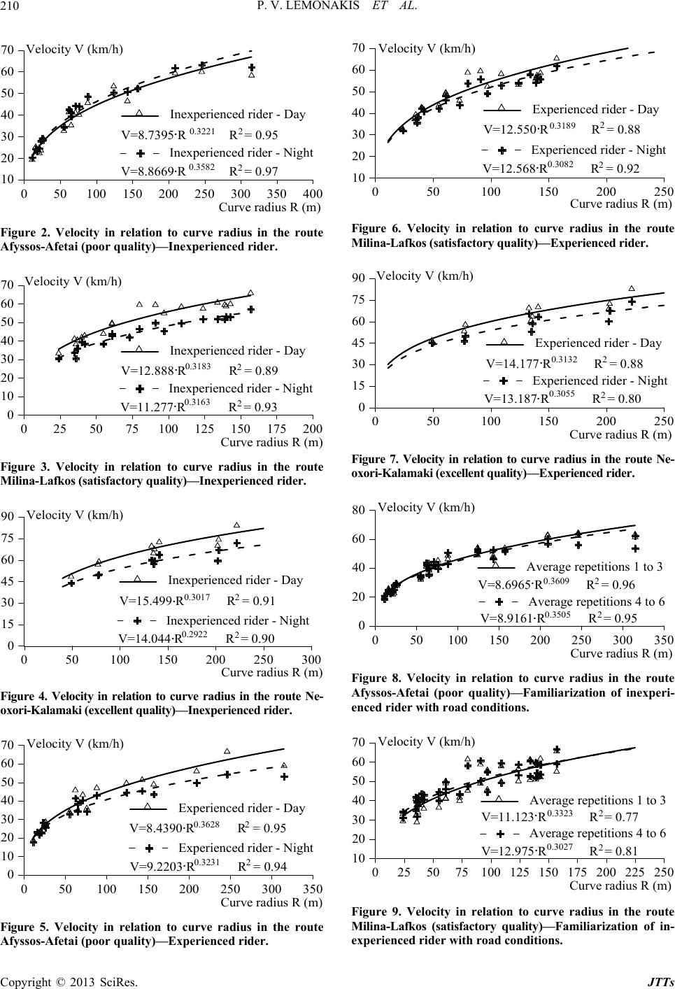

P. V. LEMONAKIS ET AL. 210
50150 250 3500100 200 300 400
10
30
50
70
20
40
60
Inexperienced rider - Day
Inexperienced rider - Night
Velocity V (km/h)
Curve radius R (m)
V=8.8669 R R = 0.97
0.3582 2
V=8.7395 R R = 0.95
0.3221 2
.
.
Figure 2. Velocity in relation to curve radius in the route
Afyssos-Afetai (poor quality)—Inexperienced rider.
2575125 175050100 150 200
10
30
50
70
0
20
40
60
Inexperienced rider - Day
Inexperienced rider - Night
Velocity V (km/h)
Curve radius R (m)
V=11.277 R R = 0.93
0.3163 2
V=12.888 R R = 0.89
0.3183 2
.
.
Figure 3. Velocity in relation to curve radius in the route
Milina-Lafkos (satisfactory quality)—Inexperienced rider.
50150 2500100 200 300
15
45
75
0
30
60
90
Inexperienced rider - Day
Inexperienced rider - Night
Velocity V (km/h)
Curve radius R (m)
V=14.044 R R = 0.90
0.2922 2
V=15.499 R R = 0.91
0.3017 2
.
.
Figure 4. Velocity in relation to curve radius in the route Ne-
oxori-Kalamaki (excellent qual ity)—I nexp erien ced r ider .
50150 250 3500100 200 300
10
30
50
70
0
20
40
60
Experienced rider - Day
Experienced rider - Night
Velocity V (km/h)
Curve radius R (m)
V=9.2203 R R = 0.94
0.3231 2
V=8.4390 R R = 0.95
0.3628 2
.
.
Figure 5. Velocity in relation to curve radius in the route
Afyssos-Afetai (poor quality)—Experienced rider.
50150 2500100200
10
30
50
70
20
40
60
Experienced rider - Day
Experienced rider - Night
Velocity V (km/h)
Curve radius R (m)
V=12.568 R R = 0.92
0.3082 2
V=12.550 R R = 0.88
0.3189 2
.
.
Figure 6. Velocity in relation to curve radius in the route
Milina-Lafkos (satisfactory quality)—Experienced rider.
501502500100 200
15
45
75
0
30
60
90
Experienced rider - Day
Experienced rider - Night
Velocity V (km/h)
Curve radius R (m)
V=13.187 R R = 0.80
0.3055 2
V=14.177 R R = 0.88
0.3132 2
.
.
Figure 7. Velocity in relation to curve radius in the route Ne-
oxori-Kalam aki (ex cellent qualit y)—Experi enced rid er.
50150 250 3500100 200 300
20
60
0
40
80
Average repetitions 1 to 3
Average repetitions 4 to 6
Velocity V (km/h)
Curve radius R (m)
V=8.9161 R R = 0.95
0.3505 2
V=8.6965 R R = 0.96
0.3609 2 .
.
Figure 8. Velocity in relation to curve radius in the route
Afyssos-Afetai (poor quality)—Familiarization of inexperi-
enced rider with road conditions.
2575125 175 225050100150 200250
10
30
50
70
20
40
60
Average repetitions 1 to 3
Average repetitions 4 to 6
Velocity V (km/h)
Curve radius R (m)
V=12.975 R R = 0.81
0.3027 2
V=11.123 R R = 0.77
0.3323 2
.
.
Figure 9. Velocity in relation to curve radius in the route
Milina-Lafkos (satisfactory quality)—Familiarization of in-
experienc e d rider with r oa d conditi ons.

P. V. LEMONAKIS ET AL. 211
50150 2500100200
15
45
75
0
30
60
90
Average repetitions 1 to 3
Average repetitions 4 to 6
Velocity V (km/h)
Curve radius R (m)
V=14 154 R R = 0.69
0.3085 2
V=15.404 R R = 0.75
0.2849 2
.
.
Figure 10. Velocity in relation to curve radius in the route
Neoxori-Kalamaki (excellent quality)—Familiarization of in-
experienc e d rider with r oa d conditi ons.
50150 250 3500100 200 300
10
30
50
70
0
20
40
60
Average repetitions 1 to 3
Average repetitions 4 to 6
Velocity V (km/h)
Curve radius R (m)
V=8.7015 R R = 0.93
0.3484 2
V=8.9442 R R = 0.92
0.3362 2
.
.
Figure 11. Velocity in relation to curve radius in the route
Afyssos-Afetai (poor quality)—Familiarization of experi-
enced rider with road conditions.
2575125 175050100150 200
10
30
50
70
0
20
40
60
Average repetitions 1 to 3
Average repetitions 4 to 6
Velocity V (km/h)
Curve radius R (m)
V=12.360 R R = 0.88
0.3255 2
V=12.799 R R = 0.85
0.3004 2
.
.
Figure 12. Velocity in relation to curve radius in the route
Milina-Lafkos (satisfactory quality)—Familiarization of ex-
perienced rider with road conditions.
50150 2500100200
15
45
75
0
30
60
90
Average repetitions 1 to 3
Average repetitions 4 to 6
Velocity V (km/h)
Curve radius R (m)
V=13.195 R R = 0.75
0.3189 2
V=14.172 R R = 0.74
0.2997 2
.
.
Figure 13. Velocity in relation to curve radius in the route
Neoxori-Kalamaki (excellent quality)—Familiarization of ex-
perienced rider with road conditions.
50150 250 3500100 200 300
10
30
50
70
0
20
40
60
80
Inexperienced rider
Experienced rider
Velocity V (km/h)
Curve radius R (m)
V=8.6167 R R = 0.95
0.3826 2
V=8.5988 R R = 0.91
0.3217 2
.
.
Figure 14. Velocity in relation to curve radius in the route
Afyssos-Afetai (poor quality)—Experienced and inexperi-
enced rider with the presence of pillion.
50150 2500100 200
10
30
50
70
20
40
60
Inexperienced rider
Experienced rider
Velocity V (km/h)
Curve radius R (m)
V=13.374 R R = 0.76
0.2861 2
V=13.210 R R = 0.78
0.2712 2
.
.
Figure 15. Velocity in relation to curve radius in the route
Milina-Lafkos (satisfactory quality)—Experienced and in-
experience d rider with the presen ce of pillion.
50150 2500100 200
10
30
50
70
90
20
40
60
80
100
Inexperienced rider
Experienced rider
Velocity V (km/h)
Curve radius R (m)
V=15.262 R R = 0.80
0.3107 2
V=16.497 R R = 0.82
0.2684 2
.
.
Figure 16. Velocity in relation to curve radius in the route
Neoxori-Kalamaki (excellent quality)—Experienced and in-
xperienced rider with t he presenc e of pillion. e

P. V. LEMONAKIS ET AL. 212
2575125 175 225 275 325050100 150 200 250 300 350
20
60
100
0
40
80
Neoxori - Kalamaki
(excellent quality)
Milina - Lafkos (satisfactory quality)
Velocity V (km/h)
Curve radius R (m)
V=12.888 R R = 0.89
0.3183 2
V=15.499 R R = 0.91
0.3017 2
Afyssos - Afetai (poor quality)
V=8.7395 R R = 0.95
2
0.3536
..
.
Figure 17. Velocity in relation to curve radius in all routes by inexperienced rider during daylight.
2575125 175 225 275325050100 150 200 250 300 350
10
30
50
70
20
40
60
80
Neoxori - Kalamaki
(excellent quality)
Milina - Lafkos (satisfactory quality)
Velocity V (km/h)
C
u
r
v
e
r
a
d
i
u
s
R
(
m
)
V=11.227 R R = 0.93
0.3163 2
V=14.044 R R = 0.90
0.2922 2
Afyssos - Afetai (poor quality)
V=8.8669 R R = 0.97
2
0.3582
..
.
Figure 18. Velocity in relation to curve radius in all routes by inexperienced rider during nightlight.
2575125 175 225 275325050100 150 200 250 300 350
10
30
50
70
20
40
60
80
Neoxori - Kalamaki
(excellent quality)
Milina - Lafkos (satisfactory quality)
Velocity V (km/h)
C
u
r
v
e
r
a
d
i
u
s
R
(
m
)
V=12.550 R R = 0.88
0.3189 2
V=14.177 R R = 0.88
0.3132 2
Afyssos - Afetai (poor quality)
V=8.4390 R R = 0.95
2
0.3628
.
.
.
Figure 19. Velocity in relation to curve radius in all routes by experienced rider during daylight.
2575125 175 225275 325050100 150 200250 300 350
15
45
75
0
30
60
90
Neoxori - Kalamaki
(excellent quality)
Milina - Lafkos (satisfactory quality)
Velocity V (km/h)
C
u
r
v
e
r
a
d
ius
R
(
m
)
V=12.568 R R = 0.92
0.3082 2
V=13.187 R R = 0.80
0.3055 2
Afyssos - Afetai (poor quality)
V=9.2203 R R = 0.94
2
0.3221
. .
Figure 20. Velocity in relation to curve radius in all routes by experienced rider during nightlight.
 In all routes, during the repetitions with the presence
of a pillion, the experienced rider speeds significant
more than the inexperienced rider (Figures 14 to 16).
(Figures 17 to 20).
REFERENCES
 Both riders either during daytime or nighttime per-
ceive the improvement of the road conditions (as de-
termined in Table 4) by increasing their velocities
[1] N. M. Islam and P. N. Seneviratne, “Evaluation of Design
Consistency of Two-Lane Rural Highways,” Institute of

P. V. LEMONAKIS ET AL. 213
Transportation Engineers Journal, Vol. 64, No. 2, 1994,
pp. 28-31.
[2] A. P. Voigt and R. A. Krammes, “An Operational and
Safety Evaluation of Alternative Horizontal Curve Design
Approaches on Rural Two-lane Highways,” Proceedings
of the International Symposium on Highway Geometric
Design Practices, Boston, 30 August-1 September 1995,
pp. 11.1-11.8.
http://onlinepubs.trb.org/onlinepubs/circulars/ec003/ch11.
pdf
[3] M. Wooldridge, K. Fitzpatrick, D. Harwood, I. Potts, L.
Elefteriadou and D. Torbic, “Geometric Design Consis-
tency on High-speed Rural Two-lane Roadways,” Trans-
portation Research Program, Washington DC, 2003.
http://onlinepubs.trb.org/onlinepubs/nchrp/nchrp_rpt_502
.pdf
[4] F. Tate and S. Turner, “Road Geometry and Drivers
Speed Choice,” Proceedings of IPENZ Transportation
Group Conference, Tauranga, 7-10 October 2007, 15p.
http://www.ipenz.org.nz/ipenztg/papers/2007/C2_TateTur
ner.pdf
[5] T. Esposito, R. Mauro, F Russo and G. Dell’Acqua,
“Speed Prediction Models for Sustainable Road Safety
Management,” Procedia—Social and Behavioral Sciences,
Vol. 20, 2011, pp. 568-576.
doi:10.1016/j.sbspro.2011.08.063
[6] S. K. Syed Abbas, M. A. Adnan and I. R. Endut, “Explo-
ration of 85th Percentile Operating Speed Model on Hor-
izontal Curve: A Case Study for Two-Lane Rural High-
ways,” Procedia—Social and Behavioral Sciences, Vol.
16, 2011, pp. 352-363. doi:10.1016/j.sbspro.2011.04.456
[7] C. R. Bennett, “A Speed Prediction Model for Rural
Two-Lane Highways,” Ph.D. Dissertation, University of
Auckland, Auckland, 1994.
[8] A. Mazzella, F. Pinna and C. Piras, “Geostatical Approach
for Operating Speed Modelling on Italian Roads,” Pro-
ceedings of the 4th International Symposium on Highway
Geometric Design, Transportation Research Board, Va-
lencia, 2-5 June 2010, 14p.
http://www.4ishgd.valencia.upv.es/index_archivos/61.pdf
[9] Y. D. Wong and A. Nicholson, “Driver Behaviour at
Horizontal Curves: Risk Compensation and the Margin of
Safety,” Accident Analysis and Prevention, Vol. 24, No. 4,
1992, pp. 425-436. doi:10.1016/0001-4575(92)90053-L
[10] Transportation Research Board, “Modeling Operating
Speed—Synthesis Report,” Washington DC, 2011.
http://onlinepubs.trb.org/onlinepubs/circulars/ec151.pdf
[11] P. Perco, “Comparison between Powered Two Wheeler
and Passenger Car Free-Flow Speeds in Urban Areas,”
Journal of the Transportation Research Board, No. 2074,
2008, pp. 77-84. doi:10.3141/2074-10
[12] S. F. Faezi, H. Hamid and S. R. Davoodi, “Predicting
Speed Model of Horizontal Curves on Exclusive Motor-
cycle Lane,” Australian Journal of Basic and Applied
Sciences, Vol. 5, No. 5, 2011, pp. 590-598.
[13] FESTA (Field opErational teSt supporT Action), “Primer
on Experimental Procedures,” 2008.
https://dspace.lboro.ac.uk/dspace-jspui/bitstream/2134/57
04/1/AR2601%20FESTA%20D2%203%20Primer%20on
%20experimental%20procedures.pdf
[14] G. Yannis, J. Golias, E. Papadimitriou and I. Spyropoulou,
“Accident Risk Analysis of Passenger Car Drivers and
Two-Wheeler Riders in Greece,” Proceedings of the 3rd
National Conference on Road Safety, Patra, 10-11 Octo-
ber 2005, 16p.
[15] S. Laporte and S. Espié (coordinators), “Understanding
Risk Taking Behaviour within the Context of PTW Rid-
ers,” 2-Wheeler Behavior & Safety—7th Framework
Program, 2011.
http://www.2besafe.eu/sites/default/files/deliverables/2BE
S_D7_SocialCognitiveAndBehaviouralDifference s OfPT W
RidersWithReferenceToTheirAttitudesTowardsRiskAndSa
fety.pdf
[16] F. G. Pratico and M. Giunta, “Operational and Safety
Effects of Two-Lane Roads Alignment,” Proceedings of
the 4th International Symposium on Highway Geometric
Design, Transportation Research Board, Valencia, 2-5
June 2010, 14p.
http://www.4ishgd.valencia.upv.es/index_archivos/73.pdf
[17] M. Castro, J. Sanchez, N. Ardila and J. Melo, “Speed
Models for Highway Consistency Analysis. A Colombian
Case Study,” Proceedings of the 4th International Sym-
posium on Highway Geometric Design, Transportation
Research Board, Valencia, 2-5 June 2010, 15p.
http://www.4ishgd.valencia.upv.es/index_archivos/28.pdf
[18] A. Abdul-Mawjoud and G. Sofia, “Development of Mod-
els for Predicting Speed on Horizontal Curves for Two-
Lane Rural Highways,” The Arabian Journal for Science
and Engineering, Vol. 33, No. 2B, 2008, pp. 365-377.
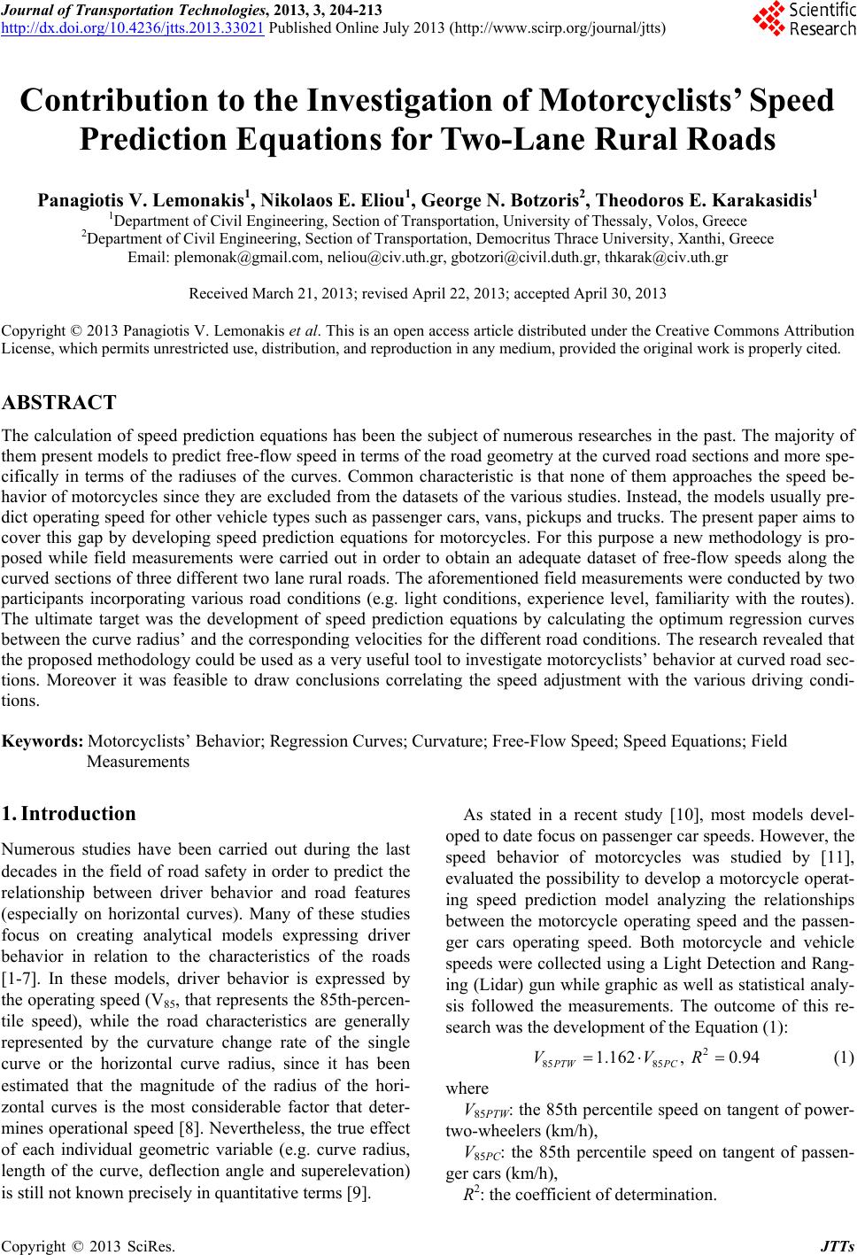