Advances in Pure Mathematics, 2013, 3, 394-404
http://dx.doi.org/10.4236/apm.2013.34057 Published Online July 2013 (http://www.scirp.org/journal/apm)
Representations of Each Number Type That Differ by
Scale Factors
Paul Benioff
Physics Division, Argonne National Laboratory, Argonne, USA
Received March 27, 2013; revised April 28, 2013; accepted May 22, 2013
Copyright © 2013 Paul Benioff. This is an open access article distributed under the Creative Commons Attribution License, which
permits unrestricted use, distribution, and reproduction in any medium, provided the original work is properly cited.
ABSTRACT
For each type of number, structures that differ by arbitrary scaling factors and are isomorphic to one another are de-
scribed. The scaling of number values in one structure, relative to the values in another structure, must be compensated
for by scaling of the basic operations and relations (if any) in the structure. The scaling must be such that one structure
satisfies the relevant number type axioms if and only if the other structure does.
Keywords: Number Types; Structures
1. Introduction
Numbers play an essential role in many areas of human
endeavor. Starting with the natural numbers, N, of ari-
thmetic, one progresses up to integers,
I
, rational num-
bers, Ra , real numbers, R, and to complex numbers,
C. In mathematics and physics, each of these types of
numbers is referred to as the natural numbers, the in-
tegers, rational numbers, real numbers, and the complex
numbers. As is well known, though, “the” means “the
same up to isomorphism” as there are many isomorphic
representations of each type of number.
In this paper, properties of different isomorphic repre-
sentations of each number type will be investigated. Em-
phasis is placed on representations of each number type
that differ from one another by arbitrary scale factors.
Here mathematical properties of these representations will
be described. The possibility that these representations
for complex numbers may be relevant to physics is de-
scribed elsewhere [1,2].
Here a mathematical system of each type is repre-
sented as a structure that satisfies a set of axioms relevant
to the type of system being considered [3,4]. A structure
consists of a base set, one or more basic operations, basic
relations (if any), and constants. Any structure containing
a base set, basic operations, relations, and constants that
are relevant for the number type, and the structure satis-
fies the relevant axioms, is a model of the axioms. As
such it is as good a representation of the number type as
is any other representation.
The contents of structures for the different types of
numbers and the chosen axiom sets are shown below:



,,,,0,1NN  Nonnegative elements of a dis-
crete ordered commutative ring with identity [5].



,,,,,0,1II Ordered integral domain [6].



,,,,,,0,1Ra Ra Smallest ordered field [7].



,,,,,,0,1RR Complete ordered field [8].



,,,,,,0,1CC   Algebraically closed field of
characteristic 0 plus axioms for complex conjugation
[9,10].
Here an overline, such as in ,N denotes a structure.
No overline, as for N, denotes a base set. The complex
conjugation operation has been added as a basic ope-
ration to C as it makes the development much easier.
For this work, the choice of which axioms are used for
each of the number types is not important. For example,
an alternate choice for N is to use the axioms of ari-
thmetic [11]. In this case N is changed by deleting the
constant 1 and adding a successor operation. There are
also other axiom choices for the real numbers [12].
The importance of the axioms is that they will be used
to show that, for two structures related by a scale factor,
one satisfies the axioms if and only if the other does.
This is equivalent to showing that one is a structure for a
given number type if and only if the other one is a struc-
ture for the same number type.
These ideas will be expanded in the following sections.
The next section gives a general treatment of fields. This
applies to all the number types that satisfy the field axi-

P. BENIOFF 395
oms (rational, real, complex numbers). However much of
the section applies to other numbers also (natural num-
bers, integers). The following five sections apply the ge-
neral results to each of the number types. The discussions
are mainly limited to properties of the number type that
are not included in the description of fields.
Section 8 expands the descriptions of the previous sec-
tions by considering ,, ,NIRaR as substructures of
.C In this case the scaling factors relating two structures
of the same type are complex numbers.
Section 9 concludes the paper with a discussion of
some aspects of number scaling, and extension to other
types of mathematical systems that are based on num-
bers.
2. General Description of Fields
It is useful to describe the results of this work for fields
in general. The results can then be applied to the different
number types, even those that are not fields. Let S be a
field structure where

,,,,,0,1.SS (1)
Here S with no overline denotes a base set, +, −, ×,
÷ denote the basic field operations, and 0,1 denote
constants. Denoting S as a field structure implies that
S is a structure that satisfies the axioms for a field [13].
Let
p
S where

,,,,,0,1.
ppppppp
SS (2)
be another structure on the same set S that is in .S
The idea is to require that p
S is also a field structure on
S where the field values of the elements of S in p S
are scaled by ,p relative to the field values in .S Here
p is a field value in .S
The goal is to show that this is possible in that one can
define p
S so that p S satisfies the field axioms if and
only if S does. To this end the notion of corres-
pondence is introduced as a relation between the field
values of p
S and .S The field value, ,
p
a in p S is
said to correspond to the field value, ,pa in .S As an
example, the identity value, 1,
p
in p S corresponds to
the value 1pp in .S
This shows that correspondence is distinct from the
concept of sameness.
p
a is the same value in p S as
a is in .S This differs from pa by the factor .p
The distinction between correspondence and sameness is
present only if 1.p If 1p

, then the two concepts
coincide, and p S and S are the same structures.
So far a scaling factor has been introduced that relates
field values between p
S and .S This must be com-
pensated for by a scaling of the basic operations in p S
relative to those of .S
The correspondences of the basic field operations and
values in p
S to those in S are given by,
,
,.
p
pp
pp
apa
p
p


 



(3)
One can use these scalings to replace the basic opera-
tions and constants in
p
S and define
p
S by,
,,, ,,0,.
p
SS pp
p

 
 



(4)
Here the subscript, ,p in ,
p
S Equation (2) is re-
placed by p as a superscript to distinguish
p
S from
.
p
S
Both
p
S and
p
S can be considered as different
representations or views of a structure that differs from
S by a scaling factor, p. A useful expression of the
relation between
p
S and
p
S is that
p
S is referred to
either as a representation of
p
S on ,S or as an explicit
representation of
p
S in terms of the operations and
element values of .S
Besides changes in the definitions of the basic opera-
tions given in Equation (3) and distinguishing between
correspondence and sameness, scaling introduces another
change. This is that one must drop the usual assumption
that the elements of the base set, ,S have fixed values,
independent of structure membership. Here the field
values of the elements of S, with one exception, depend
on the structure containing .S In particular, to say that
p
a in
p
S corresponds to pa in S means that the
element of S that has the value
p
a in
p
S has the
value pa in .S This is different from the element of
S that has the same value, ,a in S as
p
a is in .
p
S
These relations are shown schematically in Figure 1.
The valuations associated with elements in the base set
S are shown by lines from S to the structures S
and .
p
S
Figure 1. Relations between Elements in the base set
S
and their Values in the Structures
S
and
p
S
. Here
p
a
is the same value in
p
S
as a is in
S
. The lines show
that they are values for different elements of
S
. The lines
also show that the
S
element that has the value a, as
p
a in
p
S
, has the value
p
a in
S
.

P. BENIOFF 396
The one exception to the structure dependence of
valuations is the element of S with the value 0. This
value-element association is fixed and is independent of
all values of .p In this sense it is the “number vacuum”
as it is invariant under all changes pp

1.
One can define isomorphic maps between the structure
representations. Define the maps
p
W and
p
W by
.
pp
pp pp
SWSWWSFS  (5)
p
W maps S onto
p
S and
p
W maps
p
S onto
.
p
S
p
W is a map from one structure to another, and
p
W is a map between different representations of the
same structure.
p
W and
p
W are defined by

 
  
 
,
p
pppp
pppp
pppp
Wa pa
WabWaWWbpa pb
W abW aWWbpapb
p
WabWaWWbpap pb

 

 
 
(6)
and


 
    
,
.
pp
ppppppp
pppp
p
pp
pppp
ppp
Wpa a
Wpapb WpaWWpbab
WpapbWpaWWpba b
pp
W pappb W paW pWpb
ab

 
  

 
 
 

(7)
The following two theorems summarize the relations
between ,,
p
p
SS and .S The first theorem shows the
invariance of equations under the maps,
p
W and
p
W
where ,p is a scaling factor. It also shows, that the
correspondence between between element values in
p
S
and those in ,S extends to general terms.
Theorem 1 Let t and u be terms in .S Let
p
S
and
p
S be as defined in Equations (2) and (4). Then
pp
p
p
tu tut u  where ,
p
p
tWt ,
pp
uWu
and ,.
pp
p
pp p
WttWuu
Proof: It follows from the properties of
p
W and ,
p
W
Equations (6) and (7), that pp
tWtpt

 and
.
pp
uWupu Also
p
pp
tWt and .
p
pp
uWu This
gives
.
pp
pp
tutuptputu  (8)
From the left the first equation is in
p
S, the second in
,
p
S the third in both
p
S and ,S and the fourth in
.S
It remains to see in detail that the correspondence
between element values in
p
S and those in S extends
to terms. Let


,1
.
j
mp
pk
jk pp
p
a
tb




 (9)
The view of
p
t in
p
S is


,1
.
p
pj
m
p
k
jk
pa
tpb




 (10)
In the numerator, the j pa factors and 1j

mul-
tiplications contribute factors of
j
p and 1,
j
p

 res-
pectively, to give a factor p. This is canceled by a
similar factor arising from the denominator. A final
factor of p arises from the representation of the solidus
as shown in Equation (3) for division.
Using this and the fact that addition is not scaled, gives
the result that




,1 ,1
.
p
pjj
mm
p
kk
jk jk
pa a
tppt
pb b 
 

 
 

(11)
Equation (8) and the theorem follow from the fact that
Equation (11) holds for any term, including .
p
u ■
From this one has
Theorem 2
p
S sa tisfies the field axioms if and only if
p
S satisfies the field axioms if and only if S satisfies
the field axioms.
Proof: The theorem follows from Theorem 1 and the
fact that all the field axioms are equations for terms. ■
The constructions described here can be iterated. Let
p be a number value in S and
p
qq be a number
value in .
p
S Let |qp S be another field structure on the
base set, ,S and let |qp S be the representation of |qp S
using the operations and constants of
p
S2. In more
detail


|||||
,,,,0,1
qpqp qpqpqp
SS (12)
and
|,, ,,0,1.
p
qp ppp
SS qq
q



 



(13)
|qp
S is related to
p
S by the scaling factor .q The
goal is to determine the scaling factor for the
representation of |qp S on .S
To determine this, let |qp a be a value in |.
qp
S This
corresponds to a value
p
pp
qa in .
p
S Here |qp a is
the same value in |qp S as
p
pp
qa is in |qp S as
p
a
is in .
p
S
1Like the physical vacuum which is unchanged under all space time
translations.
2An equivalent way to define |qp
S is as the representation of |qp Son
.
p
S

P. BENIOFF 397
The value in S that corresponds to |qp a in |qp S
can be determined from its correspondent, ,
p
pp
qa

in
.
p
S The value in S that corresponds to
p
pp
qa

is
obtained by use of Equations (3) and (7). It is given by
 

1.
pppp
Wqa pqpapqa
p

  (14)
Here q and a are the same values in S as
p
q
and
p
a are in .
p
S Also

1,
p
W as the inverse of
,
p
W maps
p
S onto .
p
S
This is the desired result because it shows that two
steps, first with p and then with q is equivalent to
one step with .qp This result shows that the represen-
tation of |qp
S on S is given by
|,,,,0, 1. qp
SSqp qp
qp


 


(15)
Note that the steps commute in that the same result is
obtained if one scales first by q and then by p as
.pq qp Here qp is a value in .S Also this is equi-
valent to determining the scale factor for q
S on S
provided one accounts for the fact that q is a value in
p
S and not in .S
3. Natural Numbers
The natural numbers differ from the generic represen-
tation in that they are not fields [5]. This is shown by the
structure representation for ,N

,,,,0,1.NN  (16)
The structure corresponding to n
S is

,,,,0,1.
nnnnnnn
NN  (17)
Here n is any natural number 0.
One can use Equation (3) to represent n
N in terms of
the basic operations, relations, and constants of .N It is
,, ,,0,.
nn
NN n
n





(18)
Note that, as is the case for addition, the order relation
is the same in n N as in n N and in .N As was the
case for fields, n N and n N represent external and in-
ternal views of a different structure than that represented
by N. For N the external and internal views coincide.
The multiplication operator in ,
n
N n has the re-
quisite properties. This can be seen by the equivalences
between multiplication in ,,
n
n
NN and :N
.
nnn n
abc nanbncabc
n

 
Note that the simple verification of these equivalences
takes place outside the three structures and not within
any natural number structure. For this reason division by
n can be used to verify the equivalences even though it
is not part of any natural number structure.
These equivalences show that n is the multiplicative
identity in n N if and only if 1 is the multiplicative
identity in .N To see this set 1.b
The structure, ,
n
N Equation (18), and that of Equa-
tion (17), differ from the generic description, Section 2,
in that the base set n
N is a subset of .N n N contains
just those elements of N whose values in N are mul-
tiples of .n For example, the element with value n in
N has value 1 in ,
n
N and the element with value na
in N has value a in .
n
N Elements with values
na l

in N where 0,ln

 are absent from n N3.
As noted before, the choice of the representations of
the basic operations and relation and constants in ,
n
N
as shown in ,
n
N is determined by the requirement that
n
N satisfies the natural number axioms [5] if and only
if N satisfies the axioms. For the axioms that are equa-
tions and do not use the ordering relation, this follows
immediately from Theorem 1.
For axioms that use the order relation, the requirement
follows from the fact that n  and for any pair of
terms ,
nn
tu,
.
nn
n
tunt nut u

 
Here Equation (11) was used with 1.b Note that
0.n
It follows from these considerations that
Theorem 3 n N satisfies the axioms of arithmetic if
and only if n N does if and only if N does.
A simple example that illustrates the theorem is the
axiom of discreteness for the ordering,


0<1>0 1aa a

∧ [5]. One has the equiva-
lences




0< 1>01
0<>0 1
0<1>01 .
nnnnnn nn
aa a
nana nan
aa a

 

∧
∧
∧
Subscripts are missing on 0 because the value remains
the same in all structures.
4. Integers
Integers generalize the natural numbers in that negative
numbers are included. Axiomatically they can be
characterized as an ordered integral domain [6]. As a
structure, I is given by


,,,,,0,1.II (19)
I
is a base set, ,,

 are the basic operations, <
is an order relation, and 0,1 are the additive and
3The exclusion of elements of the base set in different representations
occurs only for the natural numbers and the integers. It is a conse-
quence of their not being closed under division.

P. BENIOFF 398
multiplicative identities.
Let j be a positive integer. Let
j
I
be the structure

,,,,,0,1.
j
jjjjjjj
II (20)
j
I is the subset of
I
containing all and only those
elements of
I
whose values in
I
are positive or ne-
gative multiples of j or 0.
The representation of
j
I
in terms of elements, ope-
rations, and relations in
I
is given by
,,, ,,0,.
jj
I
Ij
j
 



(21)
This structure differs from that of the natural numbers,
Equation (18), by the presence of the additive inverse,
.
The proof that
j
I
and
j
I
satisfy the integer axioms
if and only if I does, is similar to that for Theorem 3.
The only new operation is the additive inverse. Since the
axioms for this are similar to those already present,
details of the proof for axioms involving subtraction will
be skipped.
A new feature enters in the case that j is negative. It
is sufficient to consider the case where 1j as the
case for other negative integers can be described as a
combination of 1j followed by scaling with a
positive j. This would be done by extending the ite-
ration process, described for fields in Section 2, to in-
tegers.
The integer structure representations for 1j

 that
correspond to Equations (20) and (21) are given by

1111111
,,,,,0,1,II

 (22)
and
1,,,,,0,1.
1
II


 



(23)
The main thing to note here is that the order relation,
1, 
 in 1
I
 corresponds to  in .
I
1
I
 can also be described as a reflection of the whole
structure, 1
I
I through the origin at 0. Not only are
the integer values reflected but also the basic operations
and order relation are reflected. Also in this case the base
set, 1.
I
I

Equation (23) indicates that 1 is the identity and
1 is positive in 1.
I
 These follow from

1111
11
1
aaa a
 

 

and
11
01 01.


This equivalence shows that the relation, , which is
interpreted as greater than in ,
I
is interpreted as less
than in 1.
I
 Thus, as a relation in 1,
I
 01 means
1

is greater than 0. As a relation in
I
, 01
means 1

is less than 0.
This is an illustration of the relation of the ordering
relation 1 < to .< Integers which are positive in 1
I

and 1,
I

are negative in .
I
It follows that
11 111
01 2
 

 is true in 1
I
 if and only if
012  is true in 1
I
 and in .
I
These considerations show that 1
I
 and 1
I

satisfy
the integer axioms if and only if
I
satisfies the axioms.
For axioms not involving the order relation the proof is
similar to that for
j
I
for 0.j For axioms involving
the order relation the proofs proceed by restating axioms
for
I
in terms of .
An example is the axiom for transitivity
.ab bcac

∧ For this axiom the validity of the
equivalence



111111111
abbcac
ab bcac


  
∧
∧
shows that this axiom is true in 1
I if and only if it is
true in 1
I

if and only if it is true in .
I
These considerations are sufficient to show that a
theorem equivalent to Theorem 3 holds for integers:
Theorem 4 For any integer 0j,
j
I
satisfies the
integer axioms if and only if
j
I
does if and only if I
does.
5. Rational Numbers
The next type of number to consider is that of the rational
numbers. Let Ra denote a rational number structure


,,,,,,0,1.Ra Ra (24)
For each positive rational number r let r Ra denote
the structure


,,,,,,0,1.
rrrrrrrr
Ra Ra (25)
Equations (24) and (25) show that Ra and r Ra
have the same base set, .Ra This is a consequence of
the fact that rational numbers are a field. As such Ra
nd r Ra are special cases of the generic fields described
in Section 2. Note also that Ra is the same as 1.Ra
The definition of r Ra is made specific by the re-
presentation of its elements in terms of those of .Ra It
is
,,, ,,,0,.
r
Ra Rarr
r







(26)
As was seen for fields in Section 2, the number values
of the elements of Ra depend on the structure con-
taining .Ra The element of Ra that has value ra in
Ra has value a in .
r
Ra The element of Ra that
has the value a in r Ra is different from the element
that has the same value a in .Ra The only exception

P. BENIOFF 399
is the element with value 0 as this value is the same for
all .
r
Ra Also, as noted in Section 2, r Ra and r Ra
represent external and internal views of a structure that
differs from that represented by .Ra
As was the case for multiplication, the relation be-
tween rr  and  is fixed by the requirement that
r
Ra satisfy the rational number axioms [7] if and only if
r
Ra satisfies the axioms if and only if Ra does. this
can be expressed as a theorem:
Theorem 5 Let r be any nonzero rational number.
Then Ra satisfies the rational number axioms if and
only if r
Ra satisfies the axioms if and only if r Ra
does.
Proof:
Since the axioms for rational numbers include those of
an ordered field, the proof contains a combination of that
already given for fields in Section 2, Theorem 1, and for
the ordering axioms for integers, as in Theorem 4. As a
result it will not be repeated here.
It remains to prove that r
Ra is the smallest ordered
field if and only if r
Ra is if and only if Ra is. To
show this, one uses the isomorphisms defined in Section
2.
Let S be the smallest ordered field. Let r
W and
r
W be isomorphisms whose definitions on Ra and
r
Ra follow that of
p
W and
p
W in Equations (6) and
(7). That is
.
rr
rrr
Ra WRa WWRa (27)
Since these maps, as isomorphisms, are one-one onto
and are order preserving, they have inverses which are
also isomorphisms. In this case one has


r
r
rr
r
RaSW Ra RaS
WRa RaS
 

(28)
and


1
1.
r
rr
r
r
r
RaSWRa RaS
WRaRaS


 

(29)
This proves the theorem. ■
For rational number terms, Theorem 1 holds here.
From Equation (10) one sees that for rational number
structures,




,1 ,1
.
r
rjj
mm
r
kk
jk jk
ra a
trrt
rb b 
 

 
 

(30)
6. Real Numbers
The description for real numbers is similar to that for the
rational numbers. The structures Ra and ,
r
Ra Equa-
tions (24) and (25), become


,,,,,,0,1RR (31)
and


,,,,,,0,1.
r rrrrrrr
RR (32)
The external representation of the structure, whose
internal representation is ,
r
R is given in terms of the
elements, operations, relations and constants of .R It is
denoted by r R where
,,,,,,0,.
r
RRr r
r







(33)
Here r is any positive real number value in .R. If
0r

then

in Equation (33) is replaced by .
The axioms for the real numbers [8] are similar to
those for the rational numbers in that both number types
satisfy the axioms for an ordered field. For this reason
the proof that r R satisfies the ordered field axioms if
and only if r R satisfies the axioms if and only if R
does will not be given as it is essentially the same as that
for the rational numbers.
Real numbers are required to satisfy an axiom of
completeness. For this axiom, let






:0,1,2,
rr
jj
aaj be a sequence of real
numbers in ,
r
R Equation (32). Let r be a positive real
number value in R.



r
j
a converges in r R if
For all 0
rr
 there exists an h such that for all
,jm h
 
.
rrr rr
jm
r
aa (34)
Here

rrr
jm
r
aa denotes the absolute value, in
,
r
R of the difference between

r
j
a and

.
rm
a
The numerical value in ,
r
R Equation (33), that is the
same as
 
rrr
jm
r
aa is in ,
r
R is given by
.
jm
ra ra This is the same value as
j
m
aa is in
.R
j
m
ra ra also corresponds to a number value in
R given by
.
j
mjm
ra rara a
(35)
Theorem 6 Let 0r

be a real number value in .R
The sequence



r
j
a converges in r R if and only if


j
ra converges in r
R if and only if

j
a converges
in .R
Proof:
The proof is in two parts: first 0,r and then 0.r


P. BENIOFF 400
0:r Let r  be a positive number value in r
R
such that
 
.
rrr rr
jm
r
aa It follows that
jm
ra rar in both r R and .R Equation (35)
gives the result that jm aa in .R
Conversely Let jm aa be true in .R Then
jm
ra rar is true in both R and ,
r
R and
 
rrr rr
jm
r
aa is true in .
r
R From this one has
the equivalences,
 
.
rrr rrjmjm
jm
r
aa raaraa
It follows that

 r
j
a converges in r R if and only
if

j
ra converges in r
R if and only if

j
a con-
verges in .R
0r: It is sufficient to set 1.r In this case 1 R

and 1
R are given by Equations (32) and (33) with
1.r In this case

11111111
,,,,,,0,1RR

  (36)
and
1,,, ,1,,0,1.
1
RR


 



(37)
As was the case for integers, and is the case for ra-
tional numbers, this structure can also be considered as a
reflection of the structure, ,R through the origin at 0.
As before let


1
j
a be a convergent sequence in
1,R Equation (36). The statement of convergence is
given by Equation (34) where 1.r The statement
 
111 11
1
jm
aa
 

 says that
 
111
1
jm
aa


 is a positive number in 1 R

that is
less than the positive number 1

 and 0.
The corresponding statement in 1,R Equation (37),
is

1.
jm
aa

  (38)
Since 1
R is a reflection of R about the origin, the
absolute value, , in R becomes rx x

 in
1.R In 1,R the absolute value, 1,

 is always
positive even though it is always negative in .R For
example,

1
j
mjm
aa aa

  where
1
 and  are the respective absolute values
in 1 R and .R
In this case Equation (38) can be recast as
.
jm
aa  (39)
This can be used as the convergence condition in
Equation (34). Note that 0
j
m
aa  and that  de-
notes “less than or equal to” in 1.R
It follows from this that for 1,r the sequence



1
j
a converges in 1,R

Equation (36), if and only
if the sequence


j
a converges in 1,R Equation (37),
if and only if the sequence


j
a converges in .R
Extension to arbitrary negative r can be done in two
steps. One first carries out the reflection with 1r

.
This is followed by a scaling with a positive value of r
as has already been described in Section 2. ■
Theorem 7 r R is complete if and only if r R is
complete if and only if R is complete.
Proof: Assume that r
R is complete and that the
sequence



r
j
a converges in r R. Then there is a
number value r

in r R such that


lim .
j
rr
j
a

 
The properties of convergence, Equation (34), with


rm
a replaced by ,
r

and Theorem 6, can be used to
show that


limlimlim .
rr jj
j
jjj
arara

 

 (40)
Here r

is the same number value in r R as r

is
in r
R as

is in .R
Conversely assume that R is complete and that


j
a converges in R to a number value .

Repeat-
ing the above argument gives


limlimlim .
rr jj
j
jjj
arara

 

 (41)
This shows that r
R is complete if and only if r R is
complete if and only if R is complete. ■
Since real number structures are fields, Equation (11)
holds for real number terms. That is




,1 ,1
.
r
rjj
mm
r
kk
jk jk
ra a
trrt
rb b 
 


 
 

(42)
These terms can be used to give relations between
power series in ,,
r
r
RR and .R Let
 
1
,n
j
rr rr
jj
Pnxa x

 be a power series in .
r
R
Then


,
r
Pnrx and


,Pnx are the same power
series in r
R and R as

,
rr
Pnx is in .
r
R This
means that for each real number value ,
r
x


,
r
Pnrx
and


,Pnx are the respective same number values in
r
R and R as


,
rr
Pnx is in .
r
R Here rx and
x
are the same number values in r R and R as r
x
is in
.
r
R
However, the power series in R that corresponds to


,
rr
Pnx and


,
r
Pnrx in r R and r R is obtained
from Equation (11). It is




,,,.
r
rr
PnxP nrxrPnx (43)
This shows that the element of R that has value


,
rr
Pnx in r R has value

,rPn x in .R

P. BENIOFF 401
These relations extend to convergent power series.
Theorem 6 gives the result that

,
rr
Pnx is convergent
in r R if and only if

,
r
Pnrx is convergent in r R if
and only if

,rPn x is convergent in .R It follows
from Theorem 6 and Equations (40) and (41) that,
 
 
 
lim ,
lim ,
lim ,.
rrrr
n
rr
n
n
Pnxfx
Pnrxf rx
rPn xrfx






(44)
Here

rr
f
x is the same analytic function [14] in
r
R as

r
f
rx is in r R as

f
x is in .R
Equations (43) and (44) give the result that, for any
analytic function
f
,
 
.
r
rr
f
xfrxrf x (45)
Here r
f
and
f
are functions in r R and R and

rr
f
x is the same number value in r R as
 
r
f
rxrf x is in r R as

f
x is in .R Simple
examples are

ee e
rrx
xrx
rr
for the exponential and
 
sin sinsin
r
rr
x
rx rx for the sine function.
Caution:
 
22
sinsin ,
rr
x
rx not

22
sin .rx
7. Complex Numbers
The descriptions of structures for complex numbers is si-
milar to that for the real numbers. Let C denote the
complex number structure

,,,,,,0,1.CC   (46)
For each complex number c let c C be the internal
representation of another structure where

,,,,,,0,1.
c
ccccccc
CC   (47)
The external representation of the structure, in terms of
operations and constants in ,C is given by

,,, ,,,0,1.
c
CCcc c
c






(48)
The relations for the field operations are the same as
those for the real numbers except that c replaces .r It
follows that Equations (42)-(45) hold with c replacing
.r These equations show that analytic functions,

cc
f
x in ,
c
C have corresponding functions in C
given by
 
.
cc
f
xcfx (49)
Here c
x
denotes the same number in c C as
x
is in
.C
The relation for complex conjugation is given by
c
c
aca

 It is not .
c
c
aca

 One way to show this is
through the requirement that the relation for complex
conjugation must be such that 1c is a real number value
in c C if and only if 1 is a real number value in .C
This requires that the equivalences


11111 111
c
c
cc cccc




be satisfied. These equivalences show that



11
c
cc


 or more generally
 

.
cc
c
acaca

 (50)
Note that any value for a is possible including c or
powers of .c For example,


 
.
c
c
nnn
c
ccccc




As values of elements of the base set, C, Equation
(50) shows that the element of C that has value c
c
a

in
c
C has value ca

in .C This is different from the ele-
ment of C that has the same value, ,a in C as c
c
a

is in .
c
C
Another representation of the relation of complex
conjugation in c C to that in C is obtained by writing
i
e.cc

 Here c is the absolute value of .c This
can be used to write
 
2i
e.
cc
c
aca ca


 (51)
That is
 
2i
e.
c
cc






For most of the axioms, proofs that c C satisfies an
axiom if and only if C does are similar to those for the
number types already treated. However, it is worth dis-
cussing some of the new axioms. For example the
complex conjugation axiom [10]

x
x

 has an easy
proof. It is based on Equation (50), which gives







.
cc
cc
c
c
acacaca






From this one has the equivalences,

 
.
c
c
cc
aacacaaa




This shows that

x
x



is valid for c C if and
only if it is valid for c C and .C
The other axiom to consider is that for algebraic clo-
sure.
Theorem 8 c C is algebraically closed if and only if
c
C is algebraically closed if and only if C is alge-
braically closed.
Proof:
The proof consists in showing that any polynomial
equation has a solution in c C if and only if the same po-
lynomial equations in c
C and C have the same solu-
tions.
Let 00
nj
j
jbx


 denote a polynomial equation that
has a solution c a in .
c
C Then

00
j n
cc
jj
ba



in .
c
C Carrying out the replacements

,
cj
j
bcb
,
c
aca

,
cc

 and c

 gives the implications

P. BENIOFF 402
 

00
000
00
000.
c
nn
c
jj
cc j
j
jj
c
nnn
jjj
jjj
jjj
bacb ca
cbacbaba


 
 
 
 



From the left, the first equation is in ,
c
C the second
is in c C, and the other three are in .C This shows that
if c a is the solution of a polynomial in c C then ca is
the solution of the same polynomial equation in ,
c
C
and a is the solution of the same polynomial equation
in .C
The proof in the other direction consists in assuming
that 00
nj
j
jba 
 is valid in C for some number ,a
and reversing the implication directions to obtain


00
j
n
cc
jj
cba

 in .
c
C ■
8. Number Types as Substructures of c C,
c
C, and C
As is well known each complex number structure con-
tains substructures for the real numbers, the rational num-
bers, the integers, and the natural numbers. The struc-
tures are nested in the sense that each real number struc-
ture contains substructures for the rational numbers, the
integers, and the natural numbers, etc. Here it is suffi-
cient to limit consideration to the real number substruc-
tures of ,
c
C ,
c
C and C.
To this end let c be a complex number and let c R
and R be real number substructures in c C and .C In
this case

,,,,,,0,1
c cccccccc
RR (52)
and

,,,,,,0,1.RR (53)
The field operations in c R and R are the same as
those in c C and C respectively, restricted to the num-
ber values of the base sets, c
R and .R
Expression of the field operations and constants of c
R
in terms of those of C gives a representation of c
R
that corresponds to Equation (48). It is
,,, ,,,0,1.
cc
c
RRcc
c





(54)
Recall that the number values associated with the ele-
ments of a base set are not fixed but depend on the struc-
ture containing them. R contains just those elements of
C that have real values in .C c R contains just those
values of C that that have real values in c
C and .
c
C
Let
x
be an element of R that has a real value, ,a
in .R This is different from another element, ,y of
c
R that has the same real value, ,
c
a in c R as a is in
.R The element, ,y also has the value, ,ca in ,
c
R
which is the same real value in c R as a is in .R
This shows that y cannot be an element of R if c
is complex. The reason is that ca is a complex number
value in ,C and R cannot contain any elements of C
that have complex values in .C
It follows that, if c is complex, then c R and R
have no elements in common, except for the element
with value 0, which is the same in all structures.
The order relations ,
c

,
c
 and  are defined re-
lations as ordering is not a basic relation for complex
numbers. A simple definition of  in R is provided
by defining ab

in C by
if and are real number values in
and there exists a positive real number
value, , in such that .
ab C
ab
dC adb





(55)
Here d is a positive real number in C if there
exists a number
g
in C such that

.dgg

 The
definition for c

in c R is obtained by putting c sub-
scripts everywhere in Equation (55).
The order relation c

in c R is
if and are real number sin, and
there exists a positive real number
such that .
c
c
ca cbC
ca cbcd
ca cdcb





(56)
Here cd is a positive real number in c C if there
exists a number cg in c C such that

.
c
cdcg cg


One still has to prove that these definitions of ordering
are equivalent:
Theorem 9 Let ,a b be real number values in .R
Then .
cccc
abcacbab 
Proof:
Replace the three order statements by their definitions,
Eqs. 55 and 56, to get
.
ccc c
ad bcacd cbadb

  Here
dgg

,

c
cd cgcg

, and .
c
ccc
dgg


Let ,,abg be real numbers values in .R Then
,,ca cb cg and ,,
cc c
abg are the same real number
values in c R and c R as ,,ab g are in .R
Define the positive number value d by .dgg


Then by Equation (48),
g
g

is the same number value
in R as
 
c
cgcgcg gcd
c


is in c R as c
ccc
g
gd


is in .
c
R Thus cd and c d
are the same positive number values in c R and c R as
d is in .R
From this one has
,
cccc
ad bcacdcbadb



P. BENIOFF 403
which gives
.
cccc
ab cacbab 
The reverse implications are proved by starting with
,
cc
ab, and c
ccc
dgg

 and using an argument similar to
that given above. ■
9. Discussion
So far the existence of many different isomorphic struc-
ture representations of each number type has been shown.
Some properties of the different representations, such as
the fact that number values, operations, and relations, in
one representation are related to values in another repre-
sentation by scale factors have been described.
Here some additional aspects of these structure repre-
sentations and their effect on other areas of mathematics
will be briefly summarized.
One aspect worth noting is the fact that the rational,
real, and complex numbers are each both additive and
multiplicative groups. These group properties of the
fields for rational, real, and complex numbers, induce
corresponding properties in the collection of structures
for each of these number types. The discussion will be
limited to complex numbers since extension to other
number types is similar.
The map for complex numbers is
a complex number.
c
cCc
For the additive group, the map needs to be extended
to include 0r. This is done by including the empty
structure, 0.C
Let C G denote the collection of complex number
structures that differ by arbitrary nonzero complex
scaling factors. Define the operation, , by
.
cd cd
CC C (57)
Justification for this definition is provided by the
description of iteration that includes Equations (12)-(15).

GC is defined relative to the identity group structure,
,C as ,cd and cd are values in .C Every structure
c
C has an inverse, 1c C as
1. cc
CC C (58)
This shows that

GC is a multiplicative group of
complex number structures induced by the multiplicative
group of complex number values in .C Its properties
mirror the properties of the group of number values.
The additive group is defined similarly by an operation
 where .
cd cd
CCC

 The empty structure, 0 C, is
the additive identity and c
C is the additive inverse of
.
c
C
Another consequence of the existence of representa-
tions of number types that differ by scale factors is that
they affect other mathematical systems that are based on
different number types as scalars. Examples include any
system type that is closed under multiplication by nu-
merical scalars. Specific examples are vector spaces
based on either real or complex scalars, and operator al-
gebras.
For vector spaces based on complex scalars, one has
for each complex number c a corresponding pair of
structures, ,.
cc
VC The scalars for c V are number
values in .
c
C
The representation of c V as a structure with the basic
operations expressed in terms of those in ,V with C
as scalars, is similar to that for ,
c
C Equation (48). For
Hilbert spaces, the structure ,
H
based on ,C is given
by


,,,, ,,.HH

 (59)
Here

and ,

 denote scalar vector multiplica-
tion and scalar product.

denotes a general state in
.
H
The representation of another Hilbert space structure
that is based on ,
c
C is given by


,,,,, ,.
cccc c
c
HH   (60)
The representation that expresses the basic operations
of c
H
in terms of those for
H
is given by
,
,,, ,,.
c
HH c
cc


 









(61)
Additional details with c restricted to be a real num-
ber are given in [1,2].
A possible use of these structures in physics is based
on an approach to gauge theories [15,16] in which a fi-
nite dimensional vector space
x
V is associated with
each space time point .
x
So far just one complex num-
ber field, C, serves as the scalars for all the .
x
V
Expansion of this approach by replacing C with dif-
ferent complex number fields,
x
C at each point
x
has
been explored in [1,2]. If the freedom of basis choice in
the vector spaces
x
V, introduced by Yang [17], is ex-
tended to include freedom of scaling of the different
x
C,
then
y
C and
x
C are related by a scaling factor




,e.
x
y
x
yx
r 
This factor scales the numbers of
y
C relative to those
in
x
C. A number value
y
a in
y
C corresponds to the
number value ,
y
xx
ra in
x
C.
x
a is the same number
value in
x
C as
y
a is in .
y
C
The scalar field


x
 appears in gauge theories as a
scalar boson that may or may not have mass. At present
it is an open question if

is a candidate for any of the
proposed scalar fields in physics.
In any case, the scaling of number structures, and other
types of mathematical structures based on numbers,

P. BENIOFF 404
might be useful for development of a coherent theory of
physics and mathematics together [18,19]. More work
needs to be done to see if these ideas have any merit.
10. Acknowledgements
This work was supported by the US Department of
Energy, Office of Nuclear Physics, under Contract No.
DE-AC02-06CH11357.
REFERENCE
[1] P. Benioff, “New Gauge Field from Extension of Space
Time Parallel Transport of Vector Spaces to the Underly-
ing Number Systems,” International Journal of Theore-
tical Physics, Vol. 50, No. 6, 2011, pp. 1887-1907.
doi:10.1007/s10773-011-0704-3
[2] P. Benioff, “Effects on Quantum Physics of the Local
Availability of Mathematics and Space Time Dependent
Scaling Factors for Number Systems,” In: I. Ion Cotaescu,
Ed., Advances in Quantum Theory, InTech, 2012.
http://www.intechopen.com/
doi:10.5772/36485
[3] J. Barwise, “An Introduction to First Order Logic,” In: J.
Barwise, Ed., Handbook of Mathematical Logic, North-
Holland Publishing Co., New York, 1977, pp. 5-46.
doi:10.1016/S0049-237X(08)71097-8
[4] H. J. Keisler, “Fundamentals of Model Theory,” In: J.
Barwise, Ed., Handbook of Mathematical Logic, North-
Holland Publishing Co., New York, 1977, pp. 47-104.
doi:10.1016/S0049-237X(08)71098-X
[5] R. Kaye, “Models of Peano Arithmetic,” Clarendon Press,
Oxford, 1991, pp. 16-21.
[6] Wikipedia: Integral Domain.
[7] A. J. Weir, “Lebesgue Integration and Measure,” Cambri-
dge University Press, New York, 1973, p. 12.
[8] J. Randolph, “Basic Real and Abstract Analysis,” Acade-
mic Press, Inc., New York, 1968, p. 26.
[9] J. Shoenfield, “Mathematical Logic,” Addison Weseley
Publishing Co. Inc., Reading, 1967, p. 86.
[10] Wikipedia: Complex Conjugate.
[11] R. Smullyan, “Gödel’s Incompleteness Theorems,” Ox-
ford University Press,, New York, 1992, p. 29.
[12] S. Lang, “Algebra,” 3rd Edition, Addison Weseley Publi-
shing Co., Reading, 1993, p. 272.
[13] I. Adamson, “Introduction to Field Theory,” 2nd Edition,
Cambridge University Press, New York, 1982, Chapter 1.
[14] W. Rudin, “Principles of Mathematical Analysis,” 3rd
Edition, International Series in Pure and Applied Mathe-
matics, McGraw Hill Book Co., New York, 1976, p. 172.
[15] G. Mack, “Physical Principles, Geometric Aspects, and Lo-
cality Properties of Gauge Field Theories,” Fortshritte
der Physik, Vol. 29, No. 4, 1981, pp. 135-185.
doi:10.1002/prop.19810290402
[16] I. Montvay and G. Münster, “Quantum Fields on a Lat-
tice,” Cambridge Monographs on Mathematical Physics,
Cambridge University Press, Cambridge, 1994.
doi:10.1017/CBO9780511470783
[17] C. N. Yang and R. L. Mills, “Conservation of Isotopic Spin
and Isotopic Gauge Invariance,” Physic al Revi ew , Vol. 96,
No. 1, 1954, pp. 191-195. doi:10.1103/PhysRev.96.191
[18] P. Benioff, “Towards a Coherent Theory of Physics and
Mathematics,” Foundations of Physics, Vol. 32, No. 7,
2002, pp. 989-1029. doi:10.1023/A:1016561108807
[19] P. Benioff, “Towards a Coherent Cheory of Physics and
Mathematics: The Theory-Experiment Connection,” Foun-
dations of Physics, Vol. 35, No. 11, 2005, pp. 1825-1856.
doi:10.1007/s10701-005-7351-6
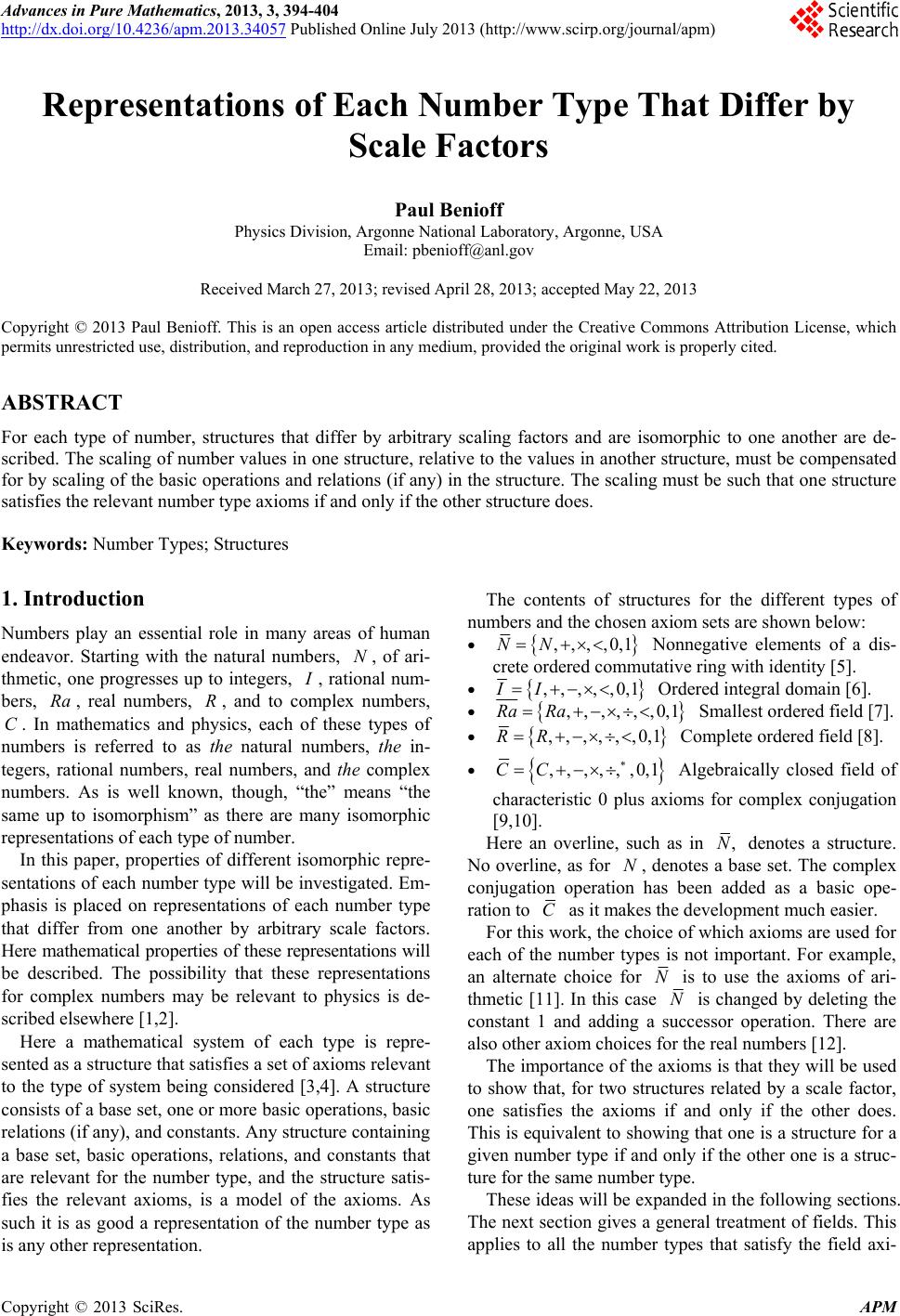