Journal of Intelligent Learning Systems and Applications, 2010, 2, 212-220
doi:10.4236/jilsa.2010.24024 Published Online November 2010 (http://www.scirp.org/journal/jilsa)
Object Identification in Dynamic Images Based on
the Memory-Prediction Theory of Brain Function
Marek Bundzel, Shuji Hashimoto
Shuji Hashimoto Laboratory, Graduate School of Advanced Science and Engineering, Waseda University, Tokyo, Japan
Received August 17th, 2010; revised September 20th, 2010; accepted September 25th, 2010.
ABSTRACT
In 2004, Jeff Hawkins presented a memory-prediction theory of brain function, and later used it to create the Hierar-
chical Temporal Memory model. Several of the concepts described in the theory are applied here in a computer vision
system for a mobile robot application. The aim was to produce a system enabling a mobile robot to explore its envi-
ronment and recognize different types of objects without human supervision. The operator has means to assign names
to the identified objects of interest. The system presented here works with time ord ered seq u ences of images. It utilizes a
tree structure of connected computational nodes similar to Hierarchical Temporal Memory and memorizes frequent
sequences of events. The structure of the proposed system and the algorithms involved are explained. A brief survey of
the existing algorithms applicable in the system is provided and future applications are outlined. Problems that can
arise when the robot’s velocity changes are listed, and a solution is proposed. The proposed system was tested on a
sequence of images recorded by two parallel cameras moving in a real world environment. Results for mono- and ste-
reo vision experiments are presented.
Keywords: Memory Prediction Framework, Mobile Robotics, Computer Vision, Unsupervised Learning
1. Introduction
This work focuses on visual data processing for use in
autonomous mobile robotics. All explanations and ex-
amples are oriented accordingly.
Humans (indeed many animals) possess the ability to
visually recognize objects in their environment thanks to
their highly developed brains. The attempts to build a
robust, multipurpose system with this ability for robots
have failed so far. Learning what the environment con-
sists of is the first step in the development of an intelli-
gent behavior.
The work described here aims to create a visual rec-
ognition system for a mobile robot. The training process
of the system is somewhat similar to the way a child
learns about the world. A child sees things and learns
about the existence of various categories of objects. No
adult trains a child to see. An adult tells the child the
names of some objects of interest so they can be referred
to in communication. The child does not learn about all
objects or their alternative appearances at once, but ra-
ther gradually increases its knowledge.
The system described here operates similarly. First,
the system collects visual data recorded at a steady
frame rate while moving around various objects. Unsu-
pervised learning is applied to identify entities in the
environment. Human operator can assign names to the
entities found. The possible advantage of such hu-
man-machine interaction is that it may be less demand-
ing than creating extensive training sets describing all
objects of interest. On the other hand, there is no direct
means to attract the attention of the system to particular
objects, and therefore the objects identified can differ
from those the operator would ideally like to obtain. The
criterion of the training is the frequency of occurrence of
spatial-temporal patterns. Therefore, anything that fre-
quently appears in the sensory input can be isolated as
an object. The unsupervised learning mechanism has
some features of the memory-prediction theory of brain
function [1].
2. Memory-Prediction Theory of Brain
Function
The memory-prediction theory of brain function was
created by Jeff Hawkins and described in the book [1].
The underlying, basic idea is that the brain is a mecha-
nism predicting the future and that hierarchical regions
of the brain predict their future input sequences.

Object Identification in Dynamic Images Based on the Memory-Prediction Theory of Brain Function 213
The theory is motivated by the observed fact that the
mammalian neocortex is remarkably uniform in appear-
ance and structure. Principally, the same hierarchical
structures are used for a wide range of behaviors, and if
necessary, the regions of the neocortex normally used for
one function can learn to perform a different task. The
memory-prediction framework provides a unified basis
for thinking about the adaptive control of complex be-
havior.
Hawkins made several assumptions [1]:
 patterns from different senses are equivalent in-
side the brain
 the same biological structures are used to process
the sensory inputs
 a single principle (a feedback/recall loop) under-
lies processing of the patterns
According to [1], discovering frequent temporal se-
quences is essential for the functioning of the brain. Pat-
terns coming from different senses are structured in both
space and time. What Hawkins considers one of the most
important concepts is that: “the cortex’s hierarchical
structure stores a model of the hierarchical structure of
the world” [1].
In the process of vision, the information moving up the
hierarchy starts as low-level retinal signals. Gradually,
increasingly complex information is extracted (presence
of sub-objects, motions, and eventually the presence of
specific objects and their corresponding behaviors). The
information moving down the hierarchy carries details
about the recognized objects and their expected behavior.
The patterns on the lower levels of the hierarchy change
quickly, and on the upper levels they change slowly.
Representations on the lower levels are spatially specific
while they become spatially invariant on the upper lev-
els.
The theory has given rise to a number of software
models aiming to simulate this common algorithm using
a hierarchical memory structure. These include an early
model [2] that uses Bayesian Networks and which served
as the foundation for later models like Hierarchical
Temporal Memory [3] or an open source project Neo-
cortex by Saulius Garalevicius [4].
3. Hierarchical Temporal Memory
Hierarchical Temporal Memory (HTM) is a machine
learning model developed by Jeff Hawkins and Dileep
George of Numenta, Inc. HTM models some of the
structural and algorithmic properties of the neocortex.
HTMs are similar to Bayesian Networks, but differ from
most in the way that time, hierarchy, action and attention
are used. The authors [3] consider the ability to discover
and infer causes to be the two most important capabili-
ties of HTM.
HTMs are organized as a tree-shaped hierarchy of
(computational) nodes. The outputs of nodes at one level
become the inputs to the next level in the hierarchy.
Nodes at the bottom of the hierarchy receive input from a
portion of the sensory input. There are more nodes in the
lower levels and fewer in the higher levels of the hierar-
chy. The output of HTM is the output of the top node.
A node works in two modes. In training mode, the
node consecutively groups spatial patterns and identifies
frequently observed temporal patterns. The grouping of
spatial patterns is performed by an algorithm for cluster
analysis. Spatial patterns are assigned to groups based on
their spatial similarity that are fewer in number than the
possible patterns, so resolution in space is lost in each
hierarchy level. A mechanism must be provided to de-
termine the probability that a new input belongs to the
identified spatial groups. Information on the membership
of the consecutive inputs to the spatial groups is recorded
in a time sequence and provides a basis for identification
of the frequently observed temporal patterns using a
Temporal Data Mining algorithm.
Despite emphasizing the importance of finding and
using frequent sequences in [1] and [3], it appears that
HTM, as initially implemented and published on the
Numenta’s website, stores only the information on spa-
tial patterns that appear frequently together and discards
the sequential information. This data structure is usually
referred to as a frequent itemset, e.g. [5]. An later
HTM-based system using a sequence memory is de-
scribed in [6]. In [6], a frequent sequence means a sub-
sequence frequently occurring in a longer sequence. This
is also known as a frequent episode, e.g. [7]. The length
of the stored frequent temporal patterns can be fixed or
variable, depending on the algorithms used and the user
settings.
In recognition mode, the node is confronted with con-
secutive inputs. Each input is assigned to one of the
stored spatial groups using the provided mechanism.
Then, the node combines this information with its previ-
ous state information and assigns a probability that the
current input is part of the stored frequent temporal pat-
terns. The output of the node is the probability distribu-
tion over the set of the stored frequent temporal patterns.
In the Numenta’s implementation of HTM, the output of
the HTM’s top node is matched with a name defined in a
training set using supervised learning, for example, a
Support Vector Machine.
4. Description of the Proposed System
4.1. Functions and Structure
Similarly to HTM, the proposed system is a hierarchy of
computational nodes, grouped into layers. A layer is a

Object Identification in Dynamic Images Based on the Memory-Prediction Theory of Brain Function
214
two dimensional rectangular grid of nodes. A node N is
identified by indices l,x,y (l is the index of the node’s
layer, x,y are the node’s coordinates within the layer).
Sensory data (either raw or preprocessed) forms the bot-
tom layer’s input matrix. The sensory data is image data
from a single or two parallel color cameras, though only
grayscale images were used here. The preprocessing can
include any filtering or image processing algorithm
which will be considered beneficial for the application.
The receptive field of a node is a rectangular portion
of its layer’s input matrix, defined by width and height.
The receptive fields of the nodes within a layer do not
overlap and together they cover the input matrix. The
receptive field of a node in the bottom layer in the
stereoscopic setup is formed as shown in Figure 1.
The stimuli in the receptive field of a node at time t
forms a vectortyxl
RF ,,, . Ordering of the elements of the
portion of the layer’s input matrix corresponding to the
receptive field of a node into a vector is arbitrary, but
must remain constant.
Output of the nodes of a layer forms the input matrix
for the layer above. The top layer contains a single node.
Output of the top node represents the output of the sys-
tem. An example of the process is given in Figure 2.
A node operates in training and recognition modes.
Training of a node is performed in two stages. The node
performs spatial grouping of the training input patterns
appearing in its receptive field by means of an algorithm
for cluster analysis (clustering). Cluster analysis is a
deeply researched domain. A survey of clustering algo-
rithms [8] provides information on categorization of the
algorithms and illustrates their applications on some da-
tasets.
The number of the identified spatial groups (clusters)
reflects the structural complexity of the input data. The
parameters of the spatial grouping algorithm of the nodes
in separate layers are likely to require different settings.
The spatial grouping algorithm must provide a mecha-
nism for categorization of a novel input.
K-means clustering [9] was used in this work. The si-
milarity measure was Euclidean distance. The training
Figure 1. Forming a receptive field of a node in the bottom
layer in the stereoscopic setup-example
Figure 2. Example, two layer hierarchy of nodes in one
time step. Layer 1 contains a single node therefore input
matrix of the Layer 1 and receptive field of the node in
Layer 1 are identical
patterns for the cluster analysis in a nde N are repre-
sented by a set
o


end
ttt RFRFRF ,...,, 1
00 . For example, if
N is in the bottom layer, the training set will contain data
representing the patterns which were appearing over time
in the portion of the image data covered by the receptive
field of N. The algorithm produces a set of k centroids


110 ,...,, 
k CCCC, where k is set by the user. The
centroids are vectors with the same number of elements
as the receptive field vector of the node.
After the spatial groups are identified, the node proc
esses the training patterns
-


end
ttt RFRFRF ,...,, 1
00 
ordered in time, starting with the oldest. Each training
pattern is assigned to exactly one spatial group. In this
work, each training pattern t RF is assigned to the spa-
tial group that has the closest centroid in terms of
Euclidean distance. The index of the winning spatial
group },...,0{, kwwt

is appended to a time ordered
list S if 1

tt ww . The node ignores repeating states
both in training and recognition modes for the reasons
explained in Section 4.2.
The time ordered list of indices (a sequence of indices)
S represents the training data for a Temporal Data Min-
ing algorithm searching for frequent episodes within S.
t represents the state of the receptive field of the node
in time t and S represents the recording of the transitions
between the states. The Temporal Data Mining algorithm
used in this work is described in [10]. It is based on the
frequent episode discovery framework [7]. It searches for
frequent episodes with variable length. The frequent
episodes identified by N are stored in a list E of
lists
w


1-Ne0 EE ,..., , where Ne is the number of the identi-
fied frequent episodes. The user determines the minimal
length of the frequent episode to be stored. It is ensured
that the shorter episodes are not contained in the longer
episodes because it would create undesired ambiguity.
There is a scale of Temporal Data Mining algorithms
related to mining for frequent temporal patterns (e.g. [7,

Object Identification in Dynamic Images Based on the Memory-Prediction Theory of Brain Function 215
11,12]) sequence matching (absolute and approximate,
e.g [14]) and sequence clustering that can be applied in a
system like the one described here. Useful surveys on
temporal data mining techniques can be found in [9] and
[10].
Operation of N in recognition mode is divided into
two consecutive stages. First, a novel input t
RF is
categorized into one of the spatial groups identified in
the training process t
twRF . If 1, t is
appended to the list BS (the buffer stack) and the oldest
item of BS is deleted. Constant length of BS is thus
maintained. BS can be seen as a short term memory be-
cause it records the recent changes of states of the recep-
tive field of the node. The length of BS is defined by the
user. The elements of BS are initialized to -1 at the start
of the algorithm. -1 does not appear in the stored fre-
quent episodes therefore BS cannot be found in any of
them before it is filled with valid values after start or
after reset.
tt ww w
Second, in the given time step, the node tries to find
which of the frequent episodes stored in E contains BS
(in direct and reverse order). The purpose is to recognize
whether the sequence of the recent changes in the recep-
tive field has been frequently observed before. The out-
put of N in time t is a binary vector t
O. The elements of
t
Ocorrespond to the stored frequent episodes. If Ei con-
tains BS in the given time step, the i-th element of t
Ois
set to 1 otherwise it is set to 0. If Ei is shorter than BS the
corresponding number of older items in BS is ignored
and the matching is performed with the shortened buffer
stack.
There are several conditions modifying the behavior
of a node in recognition mode. The node can be active
(flag A = 1) or inactive (flag A = 0), with nodes initially
starting with A = 1. The conditions are checked in each
time step. If 1 the counter Tidle is incremented
by 1.
tt ww
t
O will be equal to 1t O. If Tidle exceeds a user
defined timeout constant Tout, A is set to 0, and the ele-
ments of t O are set to 0. The node remains inactive
Table 1. Algorithms used during training (T) and recogni-
tion (R)
Algorithm Mode Comments
Data preprocessing T,R e.g. Gabor filtering, normal-
izing to unit length etc.
Clustering T
Parameters set for each layer
separately
Categorization T,R t
twRF 
Temporal data min-
ing T Parameters set for each layer separately
Sequence matching T,R finding BS in E
Name assignment T Putting a human readable
label on the objects found
until there is a significant change in its input (1

ttww).
If that happens, the node is reset: A is set to 1, Tidle is set
to 0 and the elements of BS are set to -1. This is to avoid
unrelated events lying further apart in time being consid-
ered one event by a node. For example, if only a portion
of the robot’s vision field is changing the nodes process-
ing the unchanging portion will turn inactive. This also
reduces the computational load.
Table 1 summarizes the algorithms used. Calculation
of the output t
O of a node in recognition mode in one
time step can be seen in pseudocode as follows:
{, BS, Tout, A have assigned values}
1t
w

1t
wCategorize(t
RF ,C) {Categorize current input
using the centroids}
if 1

tt ww then
if A = 0 then
1

A
end if
T
idle 1

Push(BS, wt) {Append wt to BS, delete oldest element
of BS}

t
OFindInEpisodes( BS, E) {Find which episodes
contain BS}
tt ww

1
tt OO
1
else
if A = 0 then
1
tt OO
else
1


idleidle TTTT 
if
out idle
0

A
SetAllElements(BS, -1) {Set all elements of BS
to -1}
SetAllElementst
O,0) {Set all elements of t O
to 0}
tt OO 
1
else
1 tt OO
end if
end if
end if
When BS is found to be part of a stored frequent epi-
sode, prediction of the future inputs already resides in the
remaining part of the frequent episode. The prediction
can be for example used to reduce ambiguity by catego-
rization of the incoming input if it is noisy. This feature
was not used here, however.
The user defines the structure of the hierarchy (i.e.
number of layers, dimensions of receptive fields for
nodes in each layer) and the setting of training algo-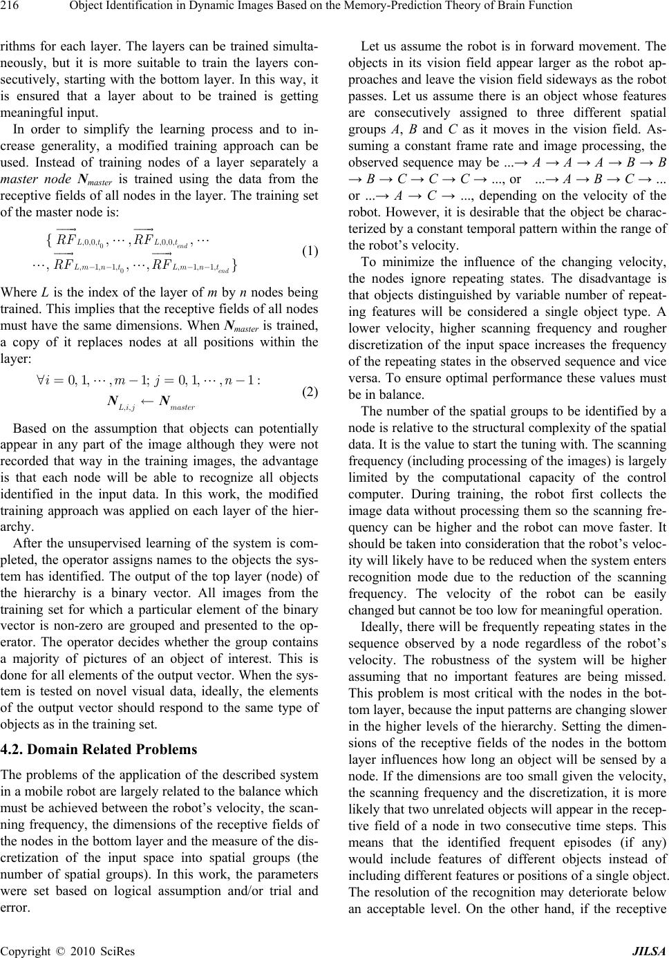

Object Identification in Dynamic Images Based on the Memory-Prediction Theory of Brain Function
216
rithms for each layer. The layers can be trained simulta-
neously, but it is more suitable to train the layers con-
secutively, starting with the bottom layer. In this way, it
is ensured that a layer about to be trained is getting
meaningful input.
In order to simplify the learning process and to in-
crease generality, a modified training approach can be
used. Instead of training nodes of a layer separately a
master node Nmaster is trained using the data from the
receptive fields of all nodes in the layer. The training set
of the master node is:
0
0
,0,0,,0,0,
,1,1, ,1,1,
{,,,
,,,
end
end
Lt Lt
Lm n tLmn t
RF RF
RF RF
---- }

 

 

(1)
Where L is the index of the layer of m by n nodes being
trained. This implies that the receptive fields of all nodes
must have the same dimensions. When Nmaster is trained,
a copy of it replaces nodes at all positions within the
layer:
NN
,,
0, 1,,1;0, 1,,1:
Li jmaster
imjn"=- =-
¬

(2)
Based on the assumption that objects can potentially
appear in any part of the image although they were not
recorded that way in the training images, the advantage
is that each node will be able to recognize all objects
identified in the input data. In this work, the modified
training approach was applied on each layer of the hier-
archy.
After the unsupervised learning of the system is com-
pleted, the operator assigns names to the objects the sys-
tem has identified. The output of the top layer (node) of
the hierarchy is a binary vector. All images from the
training set for which a particular element of the binary
vector is non-zero are grouped and presented to the op-
erator. The operator decides whether the group contains
a majority of pictures of an object of interest. This is
done for all elements of the output vector. When the sys-
tem is tested on novel visual data, ideally, the elements
of the output vector should respond to the same type of
objects as in the training set.
4.2. Domain Related Problems
The problems of the application of the described system
in a mobile robot are largely related to the balance which
must be achieved between the robot’s velocity, the scan-
ning frequency, the dimensions of the receptive fields of
the nodes in the bottom layer and the measure of the dis-
cretization of the input space into spatial groups (the
number of spatial groups). In this work, the parameters
were set based on logical assumption and/or trial and
error.
Let us assume the robot is in forward movement. The
objects in its vision field appear larger as the robot ap-
proaches and leave the vision field sideways as the robot
passes. Let us assume there is an object whose features
are consecutively assigned to three different spatial
groups A, B and C as it moves in the vision field. As-
suming a constant frame rate and image processing, the
observed sequence may be ...→ A → A → A → B → B
→ B → C → C → C → ..., or ...→ A → B → C → ...
or ...→ A → C → ..., depending on the velocity of the
robot. However, it is desirable that the object be charac-
terized by a constant temporal pattern within the range of
the robot’s velocity.
To minimize the influence of the changing velocity,
the nodes ignore repeating states. The disadvantage is
that objects distinguished by variable number of repeat-
ing features will be considered a single object type. A
lower velocity, higher scanning frequency and rougher
discretization of the input space increases the frequency
of the repeating states in the observed sequence and vice
versa. To ensure optimal performance these values must
be in balance.
The number of the spatial groups to be identified by a
node is relative to the structural complexity of the spatial
data. It is the value to start the tuning with. The scanning
frequency (including processing of the images) is largely
limited by the computational capacity of the control
computer. During training, the robot first collects the
image data without processing them so the scanning fre-
quency can be higher and the robot can move faster. It
should be taken into consideration that the robot’s veloc-
ity will likely have to be reduced when the system enters
recognition mode due to the reduction of the scanning
frequency. The velocity of the robot can be easily
changed but cannot be too low for meaningful operation.
Ideally, there will be frequently repeating states in the
sequence observed by a node regardless of the robot’s
velocity. The robustness of the system will be higher
assuming that no important features are being missed.
This problem is most critical with the nodes in the bot-
tom layer, because the input patterns are changing slower
in the higher levels of the hierarchy. Setting the dimen-
sions of the receptive fields of the nodes in the bottom
layer influences how long an object will be sensed by a
node. If the dimensions are too small given the velocity,
the scanning frequency and the discretization, it is more
likely that two unrelated objects will appear in the recep-
tive field of a node in two consecutive time steps. This
means that the identified frequent episodes (if any)
would include features of different objects instead of
including different features or positions of a single object.
The resolution of the recognition may deteriorate below
an acceptable level. On the other hand, if the receptive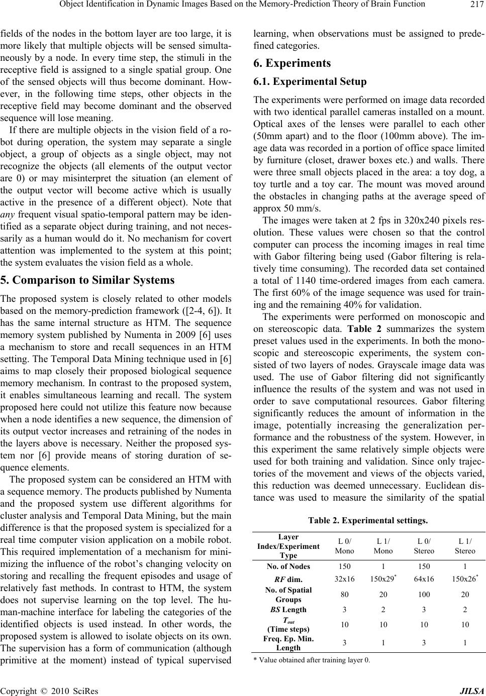

Object Identification in Dynamic Images Based on the Memory-Prediction Theory of Brain Function 217
fields of the nodes in the bottom layer are too large, it is
more likely that multiple objects will be sensed simulta-
neously by a node. In every time step, the stimuli in the
receptive field is assigned to a single spatial group. One
of the sensed objects will thus become dominant. How-
ever, in the following time steps, other objects in the
receptive field may become dominant and the observed
sequence will lose meaning.
If there are multiple objects in the vision field of a ro-
bot during operation, the system may separate a single
object, a group of objects as a single object, may not
recognize the objects (all elements of the output vector
are 0) or may misinterpret the situation (an element of
the output vector will become active which is usually
active in the presence of a different object). Note that
any frequent visual spatio-temporal pattern may be iden-
tified as a separate object during training, and not neces-
sarily as a human would do it. No mechanism for covert
attention was implemented to the system at this point;
the system evaluates the vision field as a whole.
5. Comparison to Similar Systems
The proposed system is closely related to other models
based on the memory-prediction framework ([2-4, 6]). It
has the same internal structure as HTM. The sequence
memory system published by Numenta in 2009 [6] uses
a mechanism to store and recall sequences in an HTM
setting. The Temporal Data Mining technique used in [6]
aims to map closely their proposed biological sequence
memory mechanism. In contrast to the proposed system,
it enables simultaneous learning and recall. The system
proposed here could not utilize this feature now because
when a node identifies a new sequence, the dimension of
its output vector increases and retraining of the nodes in
the layers above is necessary. Neither the proposed sys-
tem nor [6] provide means of storing duration of se-
quence elements.
The proposed system can be considered an HTM with
a sequence memory. The products published by Numenta
and the proposed system use different algorithms for
cluster analysis and Temporal Data Mining, but the main
difference is that the proposed system is specialized for a
real time computer vision application on a mobile robot.
This required implementation of a mechanism for mini-
mizing the influence of the robot’s changing velocity on
storing and recalling the frequent episodes and usage of
relatively fast methods. In contrast to HTM, the system
does not supervise learning on the top level. The hu-
man-machine interface for labeling the categories of the
identified objects is used instead. In other words, the
proposed system is allowed to isolate objects on its own.
The supervision has a form of communication (although
primitive at the moment) instead of typical supervised
learning, when observations must be assigned to prede-
fined categories.
6. Experiments
6.1. Experimental Setup
The experiments were performed on image data recorded
with two identical parallel cameras installed on a mount.
Optical axes of the lenses were parallel to each other
(50mm apart) and to the floor (100mm above). The im-
age data was recorded in a portion of office space limited
by furniture (closet, drawer boxes etc.) and walls. There
were three small objects placed in the area: a toy dog, a
toy turtle and a toy car. The mount was moved around
the obstacles in changing paths at the average speed of
approx 50 mm/s.
The images were taken at 2 fps in 320x240 pixels res-
olution. These values were chosen so that the control
computer can process the incoming images in real time
with Gabor filtering being used (Gabor filtering is rela-
tively time consuming). The recorded data set contained
a total of 1140 time-ordered images from each camera.
The first 60% of the image sequence was used for train-
ing and the remaining 40% for validation.
The experiments were performed on monoscopic and
on stereoscopic data. Table 2 summarizes the system
preset values used in the experiments. In both the mono-
scopic and stereoscopic experiments, the system con-
sisted of two layers of nodes. Grayscale image data was
used. The use of Gabor filtering did not significantly
influence the results of the system and was not used in
order to save computational resources. Gabor filtering
significantly reduces the amount of information in the
image, potentially increasing the generalization per-
formance and the robustness of the system. However, in
this experiment the same relatively simple objects were
used for both training and validation. Since only trajec-
tories of the movement and views of the objects varied,
this reduction was deemed unnecessary. Euclidean dis-
tance was used to measure the similarity of the spatial
Table 2. Experimental settings.
Layer
Index/Experiment
Type
L 0/
Mono
L 1/
Mono
L 0/
Stereo
L 1/
Stereo
No. of Nodes 150 1 150 1
RF dim. 32x16 150x29* 64x16 150x26*
No. of Spatial
Groups 80 20 100 20
BS Length 3 2 3 2
Tout
(Time steps) 10 10 10 10
Freq. Ep. Min.
Length 3 1 3 1
* Value obtained after training layer 0.

Object Identification in Dynamic Images Based on the Memory-Prediction Theory of Brain Function
218
patterns, and so changes in the cameras’ exposure setting
(over or under exposure) or a significant change in light-
ing would probably influence matching of the spatial
patterns in the bottom layer of the hierarchy negatively.
Using Gabor filtering would greatly reduce this negative
influence, but the image data was taken in a visually sta-
ble environment, a small area with dispersed light. Also,
there are simpler methods of exposure correction during
preprocessing, such as normalization of the input pat-
terns to unit length.
The relatively large receptive field of the nodes in
layer 0 ensured that the objects were sensed by a node
for several consecutive time steps and meaningful fre-
quent sequences could be identified. Using 2 fps frame
rate at the given velocity caused rapid relative movement
of the objects between consecutive images. As most of
the movement is along the horizontal axis, the width of
the receptive fields was larger than the height, so as to
capture this kind of movement.
6.2. Experimental Results
Assigning labels to the elements of the output vector of
the top node depends, to a certain extent, on the subjec-
tivity of the operator whose task it is to find a common
element in sets of pictures. For example, the majority of
pictures in a set show either the toy car or a corner of the
room or the toy car in a corner. The operator decides
whether to label the corresponding output as “the toy
car” or “a corner” or “the toy car in a corner”. Therefore,
in this case, the emphasis was on the consistency of the
results from the training and on the testing set. This
means that when the operator assigns a name to certain
outputs, these outputs will become active for the same
objects during the training and on the testing set. The use
of supervised learning is possible, but it would force the
system to find objects of predefined categories. However
the interest here was to study what objects would attract
the attention of the system.
Table 3 summarizes how many frequent episodes
were found and lengths of the episodes. Figure 3 shows
examples of the frequent episodes as sequences of cluster
centroids. It is obvious that what matters are the changes
in luminance rather than changes of texture.
Table 4 summarizes the experimental results. Varia-
tion of the information on the output of layer 1 was
lower, which confirmed expectations based on the mem-
ory-prediction theory. In the monoscopic experiment,
layer 0 transited 86 times between the identified spatial-
groups (between states) on the 640 images of the training
set. Typically, layer 0 persisted in certain states for sev-
eral time steps before it changed. This is consistent with
the fact that objects remain in the field of view for some
time before the field of view is dominated by a different
object. 8 names were assigned altogether. Groups con-
taining an uncharacteristic mixture of objects were
Table 3. Counts of frequent episodes identified in the ex-
periments
Layer Index/
Experiment Type L 0/
Mono
L 1/
Mono
L 0/
Stereo
L 1/
Stereo
Ep. Length = 1 - 20 - 20
Ep. Length = 2 - 3 - 3
Ep. Length = 3 7 1 12 0
Ep. Length = 4 12 0 8 0
Ep. Length = 5 10 0 6 0
Total 29 24 26 23
Table 4. Experimental results.
Monoscopic Experiment
Object Name Count
Train Count Test Corr. Train Corr. Test O.*
empty carpet 112 59 85% 81% 8
drawer box 38 15 79% 80% 1
car 71 42 89% 90% 4
white table 45 28 88% 89% 2
turtle 28 18 82% 83% 1
dark table 88 57 90% 79% 1
el. socket 49 21 71% 81% 1
sliding door 55 34 73% 79% 1
unidentified 198 182 - - 5
Stereoscopic Experiment
Object Name Count
Train Count Test Corr. Train Corr. Test O.*
empty carpet 105 52 74% 77% 7
drawer box 33 17 76% 76% 1
car 50 35 86% 80% 3
white table 45 28 87% 82% 3
turtle 22 15 68% 80% 2
dark table 88 57 83% 75% 1
el. socket 47 19 74% 63% 1
sliding door 55 28 78% 71% 2
unidentified 239 205 - - 3
* number of outputs responding to the object.
Figure 3. Frequent episodes 14-19 of cluster centroids
found in single camera experiment on lay er 0.

Object Identification in Dynamic Images Based on the Memory-Prediction Theory of Brain Function 219
Figure 4. Typical examples of the objects identified in the
single camera experiment. 1. “empty carpet”, 2. “drawer
box”, 3. “car”, 4. “white table”, 5. “turtle”, 6. “dark table”,
7. “corner with electric socket”, 8. “closet with sliding
door”.
designated as “unidentified”. Correctness of the output
on the testing set had to be established by manually
counting the images of the group containing the given
object. Automatic evaluation was not possible because it
was not know which objects will the system identify.
Figure 4 shows typical examples of the objects found.
In the stereoscopic experiment, the appearance of the
centroids identified at layer 0 and the overall behavior
was similar to that of the monoscopic experiment.
Therefore, the operator searched for the same objects so
that comparison would be possible. The experimental
results indicate that adding the information from the
second camera increased confusion rather than resolution.
It can be attributed to the slightly different setting of the
algorithms or to problems related to the alignment of the
cameras. In this setup, the cameras must be precisely
aligned so that the same object (shifted) will appear in
both halves of the aggregated receptive field of a node.
The confusion increased slightly more for objects near
the cameras. If an object is near the cameras, the node
may capture it only in one half of its receptive field,
loosing the depth information.
The experimental results indicate a strong consistency
between the results during the training and on the testing
sets. If there was an object identified during training, it is
very likely that the same elements of the output vector
will respond to the object on the testing set as well.
However, still a large portion of the sets are not identi-
fied, despite the presence of identified objects in the im-
ages.
7. Problems, Discussion and Future Work
One of the main problems of the system is a large num-
ber of user set parameters significantly influencing the
functioning of the system. A human operator is needed to
name the objects therefore trial and error approach is
time consuming. Algorithms for automatic optimization
of these parameters are to be developed.
Like HTM, the system can be modified for supervised
learning. A supervised learning setup can provide more
data to evaluate the behavior of the system and to de-
velop methods for optimization of the user set parame-
ters.
The algorithm matching BS with the frequent episodes
E searches for absolute match. Discretization of the input
space provides the only mean for generalization now.
Algorithm searching for approximate matches should be
employed. Also, predictions and feedback are to be im-
plemented.
The brain presumably includes information on the or-
ganism’s own movements when making predictions
about future inputs. We propose Tout to be inversely pro-
portional to the robots’ velocity in the future, to avoid
the system turning inactive if the velocity decreases or
the robot stops. Incremental learning is an important
feature of the system to be developed. Adding new fre-
quent episodes in layer L increases dimensionality of the
input matrix of the consecutive layer. Therefore the lay-
ers above L must be retrained, which requires storing the
corresponding training set. The problem considers
mainly higher levels of the hierarchy recognizing more
complex objects. If the lower levels of the hierarchy are
sufficiently trained the basic object comprising the world
has been correctly identified. More complex objects are
usually comprised from the same basic objects.
In addition to learning new sequences also forgetting
should be considered (also discussed in [4]). An
autonomous robot will presumably explore different en-
vironments and collect a large amount of knowledge.
Matching a current sequence to all of the stored frequent

Object Identification in Dynamic Images Based on the Memory-Prediction Theory of Brain Function
220
episodes would become more and more demanding over
time. We propose that frequently used sequences would
be kept active and less frequently used sequences would
be transferred into storage or completely forgotten. In the
case that a sequence is not recognized the episodes in
storage should be checked first for a possible match and
retrieved if necessary. In this way, the robot could keep
active only those learned sequences which are relevant
for the current environment.
There is no mechanism that enables the system to
identify the position of a recognized object in the image
at this point. The system usually fails if there are multi-
ple objects in the scene. We plan to develop a mecha-
nism for covert attention, presumably using feedback, to
identify the location of an object, masking it and search-
ing for other objects in the scene.
The performance of the system deteriorated slightly in
the stereoscopic experiment. The causes of the problems
mentioned in the stereoscopic experiment may be elimi-
nated by using a hierarchy with more layers and inte-
grating the information from separate cameras at higher
levels of the hierarchy, not in layer 0 directly.
Strain on the human operator is high as are the time
demands. More sophisticated means of human-system
interaction should be developed, possibly using a
mechanism for the grouping of similar images and pre-
senting only model examples to the operator and/or high-
lighting the objects in the scene that have triggered the
response.
8. Conclusions
A system for unsupervised identification of objects in
image data recorded by moving cameras in real time
using a novel combination of algorithms was presented
here. The system has some features described in mem-
ory-prediction theory of brain function. A solution was
proposed for the elimination of uncertainty linked with
the variable speed of the robot.
The system represents an early attempt to make a ma-
chine that learns largely on its own and only needs occa-
sional advice from the human operator. It is possible that
this approach may be more suitable for creating intelli-
gent multipurpose systems than trying to heavily super-
vise the learning process.
9. Acknowledgements
This work is supported by Japan Society for the Promo-
tion of Science and Waseda University, Tokyo.
REFERENCES
[1] J. Hawkins and S. Blakeslee, “On Intelligence: How a
New Understanding of the Brain Will Lead to the Crea-
tion of Truly Intelligent Machines,” Times Books, 2004,
ISBN 0-8050-7456-2
[2] D. George and J. Hawkins, “A Hierarchical Bayesian
Model of Invariant Pattern Recognition in the Visual
Cortex,” Proceedings of 2005 IEEE International Joint
Conference on Neural Networks, Vol. 3, 2005, pp. 1812-
1817.
[3] J. Hawkins and D. George, “Hierarchical Temporal
Memory-Concepts,” Theory and Terminology, White
Paper, Numenta Inc, USA, 2006.
[4] S. J. Garalevicius, “Memory-Prediction Framework for
Pattern Recognition: Performance and Suitability of the
Bayesian Model of Visual Cortex,” FLAIRS Conference,
Florida, 2007, pp. 92-97.
[5] S. Laxman and P. S. Sastry, “A Survey of Temporal Data
Mining, Sadhana,” Academy Proceedings in Engineering
Sciences, Vol. 31, No. 2, 2006, pp. 173-198.
[6] J. Hawkins, D. George and J. iemasik, “Sequence Mem-
ory for Prediction, Inference and Behaviour,” Philoso-
phical Transactions of the Royal Society B, Vol. 364, No.
1521, 2009, pp. 1203-1209.
[7] H. Mannila, H. Toivonen and A. I. Verkamo, “Discovery
of Frequent Episodes in Event Sequences,” Data Mining
Knowledge Discovery, Vol. 1, No. 1, 1997, pp. 259-289.
[8] R. Xu and D. Wunsch II, “Survey of Clustering Algo-
rithms,” IEEE Transactions on Neural Networks, Vol. 16,
No. 3, 2005, pp. 645-678.
[9] J. B. MacQueen, “Some Methods for Classification and
Analysis of Multivariate Observations,” Proceedings of
5th Berkeley Symposium on Mathematical Statistics and
Probability, Berkeley, University of California Press,
USA, 1967, pp. 281-297.
[10] D. Patnaik, P. S. Sastry and K. P. Unnikrishnan, “Infer-
ring Neuronal Network Connectivity from Spike Data: A
Temporal Data Mining Approach,” Scientific Program-
ming, Vol. 16, No. 1, 2008, pp. 49-77.
[11] R. Agrawal and R. Srikant, “Mining Sequential Patterns,”
Proceedings of 11th International Conference on Data
Engineering, Taipei, 1995, pp. 3-14.
[12] R. Agrawal, T. Imielinski and A. Swami, “A Mining
Association Rules Between Sets of Items in Large Data-
bases,” Proceedings of ACM SIGMOD Conference on
Management of Data, USA, 1993, pp. 207-216.
[13] J. Han, H. Cheng, D. Xin and X. Yan, Frequent Pattern
Mining: Current Status and Future Directions,” Data
Mining and Knowledge Discovery, Vol. 14, No. 1. 2007,
pp. 55-86.
[14] S. Wu and U. Manber, “Fast Text Searching Allowing
Errors,” Communications of the ACM, Vol. 35, No. 10,
1992, pp. 83-91.