Applied Mathematics, 2010, 1, 370-376
doi:10.4236/am.2010.15049 Published Online November 2010 (http://www.SciRP.org/journal/am)
An Improved Wavelet Based Preconditioner for Sparse
Linear Problems
Arikera Padmanabha Reddy, Nagendrapp M. Bujurke
Department of Mathematics, Karnatak University, Dharwad, India
Received August 9, 2010; revised September 11, 2010; accepted September 14, 2010
Abstract
In this paper, we present the construction of purely algebraic Daubechies wavelet based preconditioners for
Krylov subspace iterative methods to solve linear sparse system of equations. Effective preconditioners are
designed with DWTPerMod algorithm by knowing size of the matrix and the order of Daubechies wavelet. A
notable feature of this algorithm is that it enables wavelet level to be chosen automatically making it more
robust than other wavelet based preconditioners and avoids user choosing a level of transform. We demon-
strate the efficiency of these preconditioners by applying them to several matrices from Tim Davis collection
of sparse matrices for restarted GMRES.
Keywords: Discrete Wavelet Transform, Preconditioners, Sparse Matrices, Krylov Subspace Iterative
Methods
1. Introduction
The linear system of algebraic equations
A
xb (1)
where
A
is nn non-singular matrix and b is vec-
tor of size n arise while discretising differential equa-
tions using finite difference or finite element schemes.
For the solution of (1), we have a choice between direct
and iterative methods. While direct methods, such as
Gaussian elimination, can be implemented if n is small,
for very large values of n (from Tim Davis collection
of matrices [1]) it is often necessary to resort to iteration
methods such as relaxation schemes or Krylov subspace
iterative methods (Conjuagate Gradient (CG), General-
ised Minimum Residual (GMRES) and their variants etc).
Each iterative method is aimed at providing a way of
solving a particular class of linear system, but none can
be relied upon to perform well for all problems. Usually
it is necessary to make use of a preconditioner to accel-
erate the convergence of iteration. This means that the
original system of equations is transformed into equiva-
lent system, which is more amenable to solution by a
chosen iterative method (Ford [2]). The combination of
preconditioning and Krylov subspace iterations could
provide efficient and simple general-purpose procedures
that compete with direct solvers (Saad [3]). A precondi-
tioner is a non-singular matrix ()PA with 1 P
A
I


.
The philosophy is that the preconditioner has to be close
to
A
and still allow fast converging iteration. The
broad class of these preconditioners are mainly obtained
by splitting
A
, say, in the form
A
PQ and writing
(1) in the form


11
.
I
PQx Pb

 (2)
If P is the diagonal of
A
then the iteration scheme
is due to Jacobi (P is not close to
A
) and the other ex-
treme is PA

(too close to
A
). In between these two
extremities, we look for Pas band matrix constructed
by setting to zero all entries of the matrix outside a cho-
sen diagonal bandwidth [4].
Discrete Wavelet Transform (DWT) is a big boon es-
pecially in signal and Image processing where in smooth
data can be compressed sufficiently without loosing pri-
mary features of the data. Compressed data either thre-
sholding or cutting is of much use if we are not using it
in further process such as using it as preconditioner.
DWT results in matrices with finger pattern. If DWT is
followed by the permutation of the rows and columns of
the matrix then it centres/brings the finger pattern about
the leading diagonal. This strategy is termed as DWTPer
an elegant analysis presented by Chen [5,6] for large
dense matrices which enables in predicting the width of

A. P. REDDY ET AL. 371
band of matrix. Later, an approximate form of this can be
formed and taken as preconditioner, which controls fill-
in whenever schemes like LUdecomposition is used.
Similar criteria is adopted in transforming non-smooth
parts, if any, which are horizontal/vertical bands and are
shifted to the bottom and right-hand edges of the matrix
after applying DWTPer. This procedure is termed as
DWTPerMod [7] and takes care of other cases where
non-smooth parts are located in the matrix. This scheme
is more effective in incorporating missing finer details
such as fixing of precise bandwidth and automatic selec-
tion of choice of transform level. Using DWTPerMod
algorithm Ford [7] has presented its salient features by
applying it to standard dense matrices arising in various
disciplines/fields of interest.
Kumar and Mehra [8] use iDWT, iDWTPer (imple-
mentation of DWT by zero padding [9]) and demonstrate
their efficiency as preconditioner for ill conditioned
sparse matrices and iDWTPer to be more robust precon-
ditioners for sparse systems. Motivated by this work
([5-8]), we have successfully used DWTPerMod algo-
rithm in selecting the level of wavelet transform auto-
matically by knowing the size of the matrix, order of
wavelet used and construct effective preconditioner for
sparse unsymmetric linear systems.
The structure of the paper is organised as follows: In
Section 2 we explain briefly about orthogonal wavelets.
Section 3 contains practical computation details of tran-
sforms required. Here, we present the main results of
wavelet based preconditioners in the form of Theorem
and Algorithms. In Section 4 we illustrate seven typical
test problems selected from Tim Davis collection to em-
phasize the potential usefulness of preconditioners de-
signed using various orders of Daubechies wavelet. Fi-
nally, in Section 5 we summarise our conclusion and
give future plan of work.
2. Wavelet Preliminaries
The effective introduction to wavelets via multiresolu-
tion analysis (MRA) is broad based compared with con-
ventional/classical way through scaling function concept
and as such the following basics are given below.
2.1. Multiresolution Analysis
A multire solution analysis [9-11] on R is a sequence
of closed subspaces

j
j
V of

2
LR satisfying the
following conditions
1) nestedness: 1
j
j
VV


2) completeness: closure of j V


2
LR, nullity:

0
j
V

3) scale invariance:


1
2
j
j
f
xV fxV


4) shift invariance:


00
,
f
xV fxkVkZ 
5) shift invariant basis: there exists function

in 0 V
whose integer translates



k   are an orthonormal
basis for 0 V.
Let 0 Wbe a complement of 0 V in1 V, i.e.,
10 0
VV W

. This implies that there exists a function
0
W


such that its translates
 
k
k 

 are an
orthonormal basis for0 W. For each,jk Z, define



2
,22
jj
jk
x
xk 





2
,22
jj
jk
x
xk 


then these form orthonormal bases for and
j
j
VW re-
spectively and


,/, nk nk Z
 forms an orthonormal
basis of


2
LR and
1
j
jj
VVW
 (3)
Since 0 V and 0 Ware contained in 1 V, we have



 
22, 22
kk
kk
x
hxk xgxk  

 


for some




,
kk
hgin

2
lR. Here



,
kk
hg are
called lowpass and highpass filter coefficients respec-
tively. These filter coefficients can be generated using
factorization scheme of Daubechies polynomials [11,12]
and the functions and

 are called scaling and wave-
let functions respectively. We define orthogonal projec-
tions ,
j
j
PQ from


2
LR onto ,
j
j
VW by
,,
,.
j
jk jk
k
Pf f






(4)
1,,
,..
j
jjjk jk
k
QfP fPff 




j
P and
j
Qare also called approximation and detail
operators on
f
and for any

2
f
LR, j Pf fin
2
Las j .
3. Practical Computations
Suppose that a vector (signal) sfrom a vector spacen
R
is given. One may construct it as an infinite sequence by
extending the signal by periodic form/extension [9,11]
and use this extended signal as a sequence of scaling
coefficients for some underlying function
L
f
in some
fixed space
L
Vof 2 L(from (4)) as


,,LLkLk
k
f
xs x  

. (5)
From (3), we have 11 ...
L
rrr L
VVWW W

,
this implies that
 
1
,, ,,
L
Lrkrk titi
ktri
f
xs xdx 




. (6)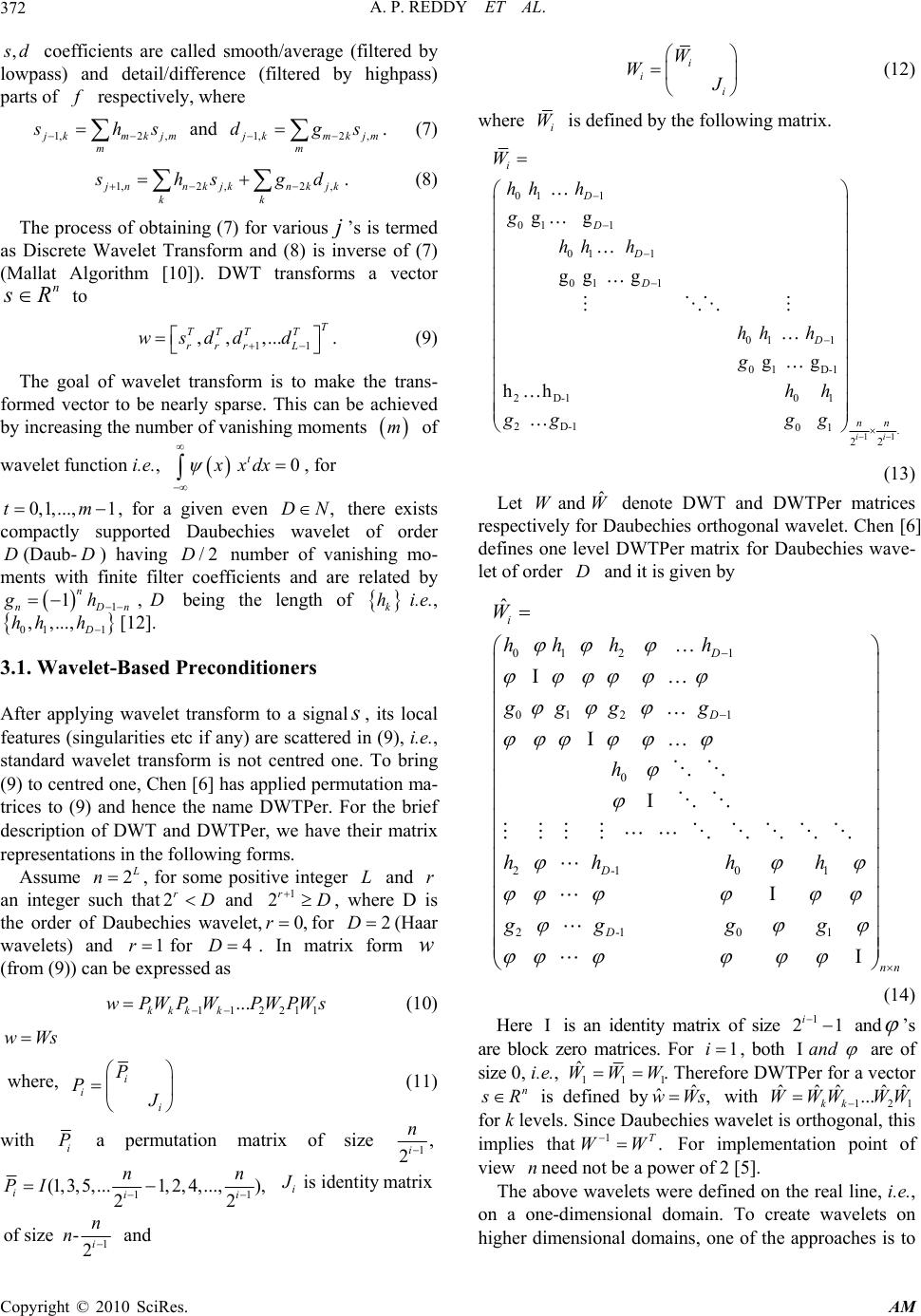

A. P. REDDY ET AL. 372
,
s
d coefficients are called smooth/average (filtered by
lowpass) and detail/difference (filtered by highpass)
parts of f respectively, where
1,2 ,
j
kmkjm
m
s
hs

 and 1,2 ,
j
kmkjm
m
dgs

. (7)
1,2 ,2,
j
nnkjknkjk
kk
s
hs gd



. (8)
The process of obtaining (7) for various
j
’s is termed
as Discrete Wavelet Transform and (8) is inverse of (7)
(Mallat Algorithm [10]). DWT transforms a vector
n
sR to
11
,, ,....
T
TTT T
rrr L
wsdd d



(9)
The goal of wavelet transform is to make the trans-
formed vector to be nearly sparse. This can be achieved
by increasing the number of vanishing moments


m of
wavelet function i.e.,

0
t
xxdx 



, for
0,1,..., 1tm, for a given even ,DN there exists
compactly supported Daubechies wavelet of order
D(Daub- D) having /2D number of vanishing mo-
ments with finite filter coefficients and are related by

1
1n
nDn
gh

 ,D being the length of


k
hi.e.,

01 1
,,..., D hh h
[12].
3.1. Wavelet-Based Preconditioners
After applying wavelet transform to a signals, its local
features (singularities etc if any) are scattered in (9), i.e. ,
standard wavelet transform is not centred one. To bring
(9) to centred one, Chen [6] has applied permutation ma-
trices to (9) and hence the name DWTPer. For the brief
description of DWT and DWTPer, we have their matrix
representations in the following forms.
Assume 2
L
n, for some positive integer L and r
an integer such that1
2 and 2
rr
DD

, where D is
the order of Daubechies wavelet,0,rfor 2D

(Haar
wavelets) and 1rfor 4D

. In matrix form w
(from (9)) can be expressed as
112211
...
kkk k
wPWPWPWPWs

 (10)
wWs
where, i
i
i
P
P
J



(11)
with i P a permutation matrix of size 1,
2i
n

11
(1,3,5,...1, 2, 4,...,),
22
iii
nn
PI   is identity matrix
i
J
1
of size -2i
n
n and
i
i
i
W
W
J



(12)
where i W is defined by the following matrix.
01 1
01 1
01 1
01 1
01 1
01 D-1
2D-1 01
2D-1 01
g g
g g g
g g
hh
i
D
D
D
D
D
W
hh h
g
hh h
hh h
g
hh
gg gg






























11
.
22
ii
nn





(13)
Let ˆ
and WW denote DWT and DWTPer matrices
respectively for Daubechies orthogonal wavelet. Chen [6]
defines one level DWTPer matrix for Daubechies wave-
let of order D and it is given by
0121
01 21
0
ˆ
i
D
D
W
hh hh
gg gg
h
 












2-1 01
2-1
D
D
hh hh
gg


 




  


01
nn
gg 
 





















(14)
Here

is an identity matrix of size 1 21
i and

’s
are block zero matrices. For 1i, both and

 are of
size 0, i.e., 11
1
ˆ
WW
W

. Therefore DWTPer for a vector
n
s
R is defined byˆ
ˆ,
wWs with 121
ˆˆˆˆˆ
...
kk
WWWWW


for k levels. Since Daubechies wavelet is orthogonal, this
implies that1.
T
WW
 For implementation point of
view nneed not be a power of 2 [5].
The above wavelets were defined on the real line, i.e.,
on a one-dimensional domain. To create wavelets on
higher dimensional domains, one of the approaches is to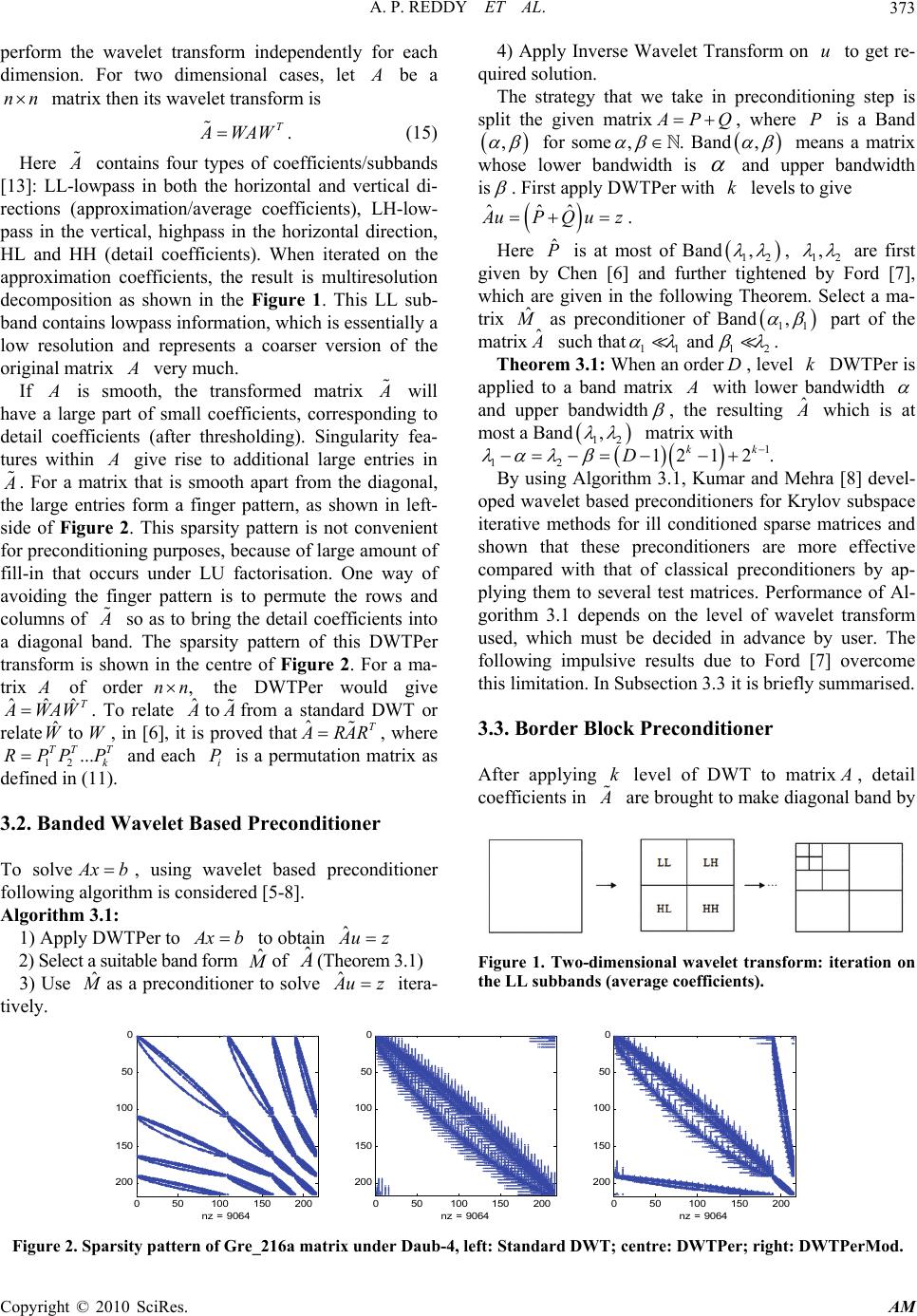

A. P. REDDY ET AL. 373
perform the wavelet transform independently for each
dimension. For two dimensional cases, let
A
be a
nn matrix then its wavelet transform is
T
A
WAW
. (15)
Here
A
 contains four types of coefficients/subbands
[13]: LL-lowpass in both the horizontal and vertical di-
rections (approximation/average coefficients), LH-low-
pass in the vertical, highpass in the horizontal direction,
HL and HH (detail coefficients). When iterated on the
approximation coefficients, the result is multiresolution
decomposition as shown in the Figure 1. This LL sub-
band contains lowpass information, which is essentially a
low resolution and represents a coarser version of the
original matrix
A
very much.
If
A
is smooth, the transformed matrix
A
 will
have a large part of small coefficients, corresponding to
detail coefficients (after thresholding). Singularity fea-
tures within
A
give rise to additional large entries in
A
. For a matrix that is smooth apart from the diagonal,
the large entries form a finger pattern, as shown in left-
side of Figure 2. This sparsity pattern is not convenient
for preconditioning purposes, because of large amount of
fill-in that occurs under LU factorisation. One way of
avoiding the finger pattern is to permute the rows and
columns of
A
 so as to bring the detail coefficients into
a diagonal band. The sparsity pattern of this DWTPer
transform is shown in the centre of Figure 2. For a ma-
trix
A
of order,nn the DWTPer would give
ˆˆˆ
T
A
WAW. To relate ˆ to
A
A
from a standard DWT or
relate ˆ to WW , in [6], it is proved thatˆT
A
RAR, where
12
...
TT T
k
RPP P and each i P is a permutation matrix as
defined in (11).
3.2. Banded Wavelet Based Preconditioner
To solve
A
xb, using wavelet based preconditioner
following algorithm is considered [5-8].
Algorithm 3.1:
1) Apply DWTPer to
A
xb to obtain ˆ
A
uz

2) Select a suitable band form ˆ
M
of ˆ
A
(Theorem 3.1)
3) Use ˆ
M
as a preconditioner to solve ˆ
A
uz

itera-
tively.
4) Apply Inverse Wavelet Transform on u to get re-
quired solution.
The strategy that we take in preconditioning step is
split the given matrix
A
PQ

, where P is a Band


,

 for some,




. Band

,

 means a matrix
whose lower bandwidth is

and upper bandwidth
is

. First apply DWTPer with k levels to give


ˆˆ
ˆ
A
uPQuz

.
Here ˆ P is at most of Band

12
,

 , 12 ,

 are first
given by Chen [6] and further tightened by Ford [7],
which are given in the following Theorem. Select a ma-
trix ˆ
M
as preconditioner of Band

11
,

 part of the
matrix ˆ
A
such that11 12 and

 .
Theorem 3.1: When an orderD, level k DWTPer is
applied to a band matrix
A
with lower bandwidth

and upper bandwidth

, the resulting ˆ
A
which is at
most a Band


12
,

 matrix with




1
12 1212 .
kk
D  

 
By using Algorithm 3.1, Kumar and Mehra [8] devel-
oped wavelet based preconditioners for Krylov subspace
iterative methods for ill conditioned sparse matrices and
shown that these preconditioners are more effective
compared with that of classical preconditioners by ap-
plying them to several test matrices. Performance of Al-
gorithm 3.1 depends on the level of wavelet transform
used, which must be decided in advance by user. The
following impulsive results due to Ford [7] overcome
this limitation. In Subsection 3.3 it is briefly summarised.
3.3. Border Block Preconditioner
After applying k level of DWT to matrix
A
, detail
coefficients in
A
 are brought to make diagonal band by
Figure 1. Two-dimensional wavelet transform: iteration on
the LL subbands (average coefficients).
050100150200
0
50
100
150
200
nz = 9064
050100 150 200
0
50
100
150
200
nz = 9064
050100150 200
0
50
100
150
200
nz = 9064
Figure 2. Sparsity pattern of Gre_216a matrix under Daub-4, left: Standard DWT; centre: DWTPer; right: DWTPerMod.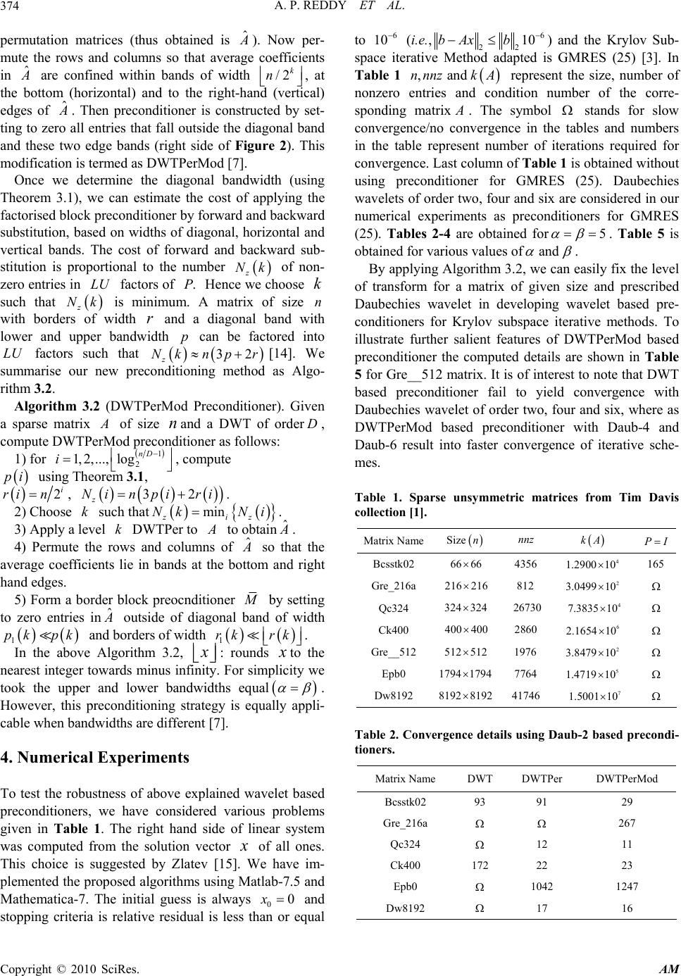

A. P. REDDY ET AL. 374
permutation matrices (thus obtained is ˆ
A
). Now per-
mute the rows and columns so that average coefficients
in ˆ
A
are confined within bands of width /2
k
n


, at
the bottom (horizontal) and to the right-hand (vertical)
edges of ˆ
A
. Then preconditioner is constructed by set-
ting to zero all entries that fall outside the diagonal band
and these two edge bands (right side of Figure 2). This
modification is termed as DWTPerMod [7].
Once we determine the diagonal bandwidth (using
Theorem 3.1), we can estimate the cost of applying the
factorised block preconditioner by forward and backward
substitution, based on widths of diagonal, horizontal and
vertical bands. The cost of forward and backward sub-
stitution is proportional to the number

z
Nk
of non-
zero entries in LU factors of .P Hence we choose k
such that

z
Nk
is minimum. A matrix of size n
with borders of width r and a diagonal band with
lower and upper bandwidth p can be factored into
LU factors such that

 
32
z
Nkn pr [14]. We
summarise our new preconditioning method as Algo-
rithm 3.2.
Algorithm 3.2 (DWTPerMod Preconditioner). Given
a sparse matrix
A
of size nand a DWT of orderD,
compute DWTPerMod preconditioner as follows:
1) for

1
2
1, 2,...,lognD i

 , compute

pi using Theorem 3.1,

2i ri n,


32
z
Nin piri .
2) Choose k such that



min
ziz
Nk Ni.
3) Apply a level k DWTPer to
A
to obtainˆ
A
.
4) Permute the rows and columns of ˆ
A
so that the
average coefficients lie in bands at the bottom and right
hand edges.
5) Form a border block preocnditioner
M
by setting
to zero entries in ˆ
A
outside of diagonal band of width

1
pk pk and borders of width



1
rk rk 

.
In the above Algorithm 3.2,
x


: rounds
x
to the
nearest integer towards minus infinity. For simplicity we
took the upper and lower bandwidths equal



 .
However, this preconditioning strategy is equally appli-
cable when bandwidths are different [7].
4. Numerical Experiments
To test the robustness of above explained wavelet based
preconditioners, we have considered various problems
given in Table 1. The right hand side of linear system
was computed from the solution vector
x
of all ones.
This choice is suggested by Zlatev [15]. We have im-
plemented the proposed algorithms using Matlab-7.5 and
Mathematica-7. The initial guess is always 00x

and
stopping criteria is relative residual is less than or equal
to 6
10

(i.e.,6
22
10bAxb   ) and the Krylov Sub-
space iterative Method adapted is GMRES (25) [3]. In
Table 1


, and nnnzk A represent the size, number of
nonzero entries and condition number of the corre-
sponding matrix
A
. The symbol  stands for slow
convergence/no convergence in the tables and numbers
in the table represent number of iterations required for
convergence. Last column of Table 1 is obtained without
using preconditioner for GMRES (25). Daubechies
wavelets of order two, four and six are considered in our
numerical experiments as preconditioners for GMRES
(25). Tables 2-4 are obtained for5

 
. Table 5 is
obtained for various values of and

 .
By applying Algorithm 3.2, we can easily fix the level
of transform for a matrix of given size and prescribed
Daubechies wavelet in developing wavelet based pre-
conditioners for Krylov subspace iterative methods. To
illustrate further salient features of DWTPerMod based
preconditioner the computed details are shown in Table
5 for Gre__512 matrix. It is of interest to note that DWT
based preconditioner fail to yield convergence with
Daubechies wavelet of order two, four and six, where as
DWTPerMod based preconditioner with Daub-4 and
Daub-6 result into faster convergence of iterative sche-
mes.
Table 1. Sparse unsymmetric matrices from Tim Davis
collection [1].
Matrix NameSize


n nnz

kA
P
I

Bcsstk02 6666

4356 4
1.290010 165
Gre_216a 216 216

812 2
3.0499 10

Qc324 324324

26730 4 7.383510

Ck400 400 400

2860 6
2.1654 10

Gre__512 512 512

1976 2
3.8479 10

Epb0 17941794

7764 5
1.471910

Dw8192 8192 8192

41746 7
1.500110

Table 2. Convergence details using Daub-2 based precondi-
tioners.
Matrix Name DWT DWTPer DWTPerMod
Bcsstk02 93 91 29
Gre_216a

 267
Qc324

12 11
Ck400 172 22 23
Epb0

1042 1247
Dw8192

17 16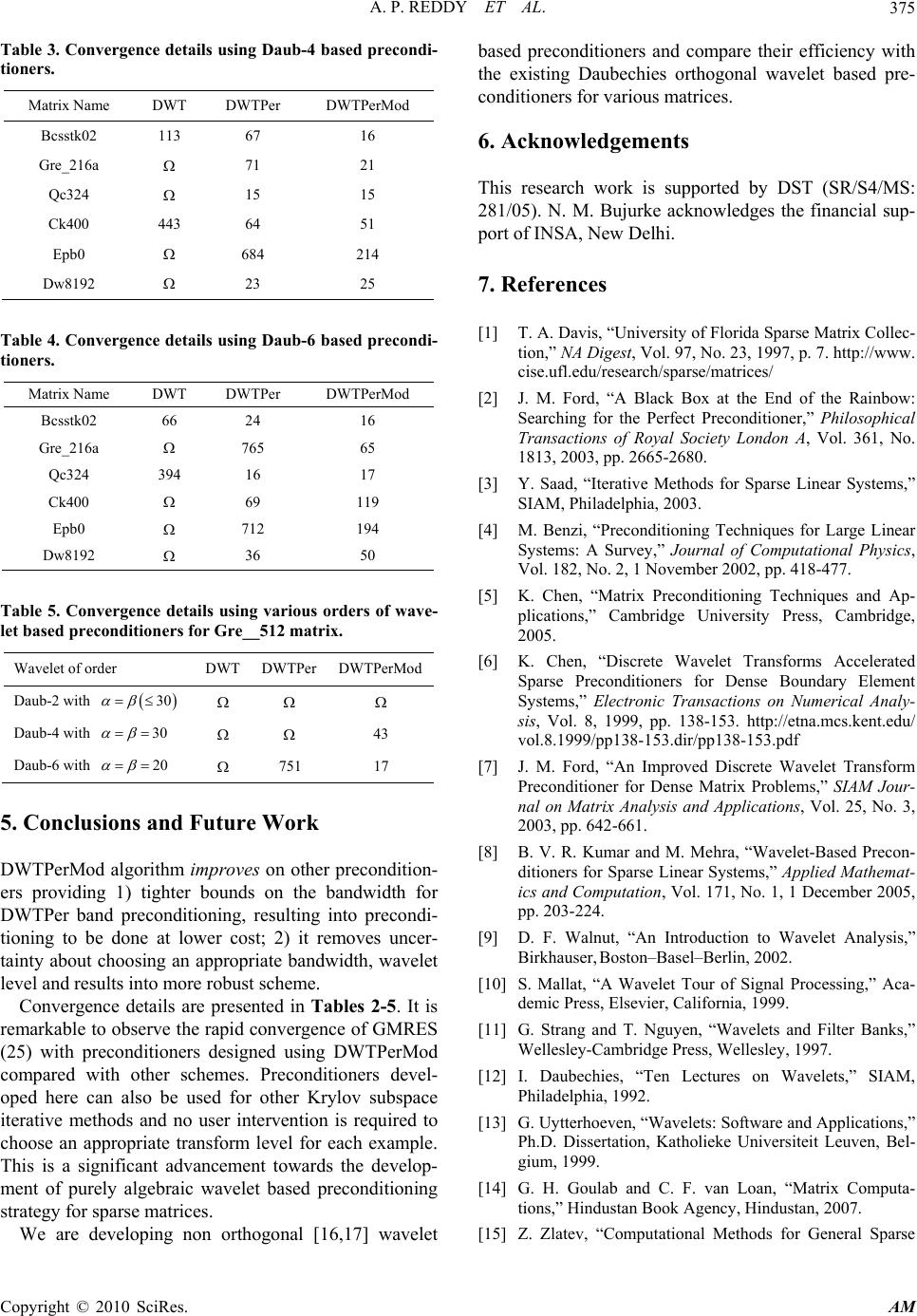

A. P. REDDY ET AL. 375
Table 3. Convergence details using Daub-4 based precondi-
tioners.
Matrix Name DWT DWTPer DWTPerMod
Bcsstk02 113 67 16
Gre_216a  71 21
Qc324  15 15
Ck400 443 64 51
Epb0  684 214
Dw8192  23 25
Table 4. Convergence details using Daub-6 based precondi-
tioners.
Matrix Name DWT DWTPer DWTPerMod
Bcsstk02 66 24 16
Gre_216a  765 65
Qc324 394 16 17
Ck400  69 119
Epb0  712 194
Dw8192  36 50
Table 5. Convergence details using various orders of wave-
let based preconditioners for Gre__512 matrix.
Wavelet of order DWTDWTPer DWTPerMod
Daub-2 with 
30    

Daub-4 with 30

    43
Daub-6 with 20

   751 17
5. Conclusions and Future Work
DWTPerMod algorithm improves on other precondition-
ers providing 1) tighter bounds on the bandwidth for
DWTPer band preconditioning, resulting into precondi-
tioning to be done at lower cost; 2) it removes uncer-
tainty about choosing an appropriate bandwidth, wavelet
level and results into more robust scheme.
Convergence details are presented in Tables 2-5. It is
remarkable to observe the rapid convergence of GMRES
(25) with preconditioners designed using DWTPerMod
compared with other schemes. Preconditioners devel-
oped here can also be used for other Krylov subspace
iterative methods and no user intervention is required to
choose an appropriate transform level for each example.
This is a significant advancement towards the develop-
ment of purely algebraic wavelet based preconditioning
strategy for sparse matrices.
We are developing non orthogonal [16,17] wavelet
based preconditioners and compare their efficiency with
the existing Daubechies orthogonal wavelet based pre-
conditioners for various matrices.
6. Acknowledgements
This research work is supported by DST (SR/S4/MS:
281/05). N. M. Bujurke acknowledges the financial sup-
port of INSA, New Delhi.
7. References
[1] T. A. Davis, “University of Florida Sparse Matrix Collec-
tion,” NA Digest, Vol. 97, No. 23, 1997, p. 7. http://www.
cise.ufl.edu/research/sparse/matrices/
[2] J. M. Ford, “A Black Box at the End of the Rainbow:
Searching for the Perfect Preconditioner,” Philosophical
Transactions of Royal Society London A, Vol. 361, No.
1813, 2003, pp. 2665-2680.
[3] Y. Saad, “Iterative Methods for Sparse Linear Systems,”
SIAM, Philadelphia, 2003.
[4] M. Benzi, “Preconditioning Techniques for Large Linear
Systems: A Survey,” Journal of Computational Physics,
Vol. 182, No. 2, 1 November 2002, pp. 418-477.
[5] K. Chen, “Matrix Preconditioning Techniques and Ap-
plications,” Cambridge University Press, Cambridge,
2005.
[6] K. Chen, “Discrete Wavelet Transforms Accelerated
Sparse Preconditioners for Dense Boundary Element
Systems,” Electronic Transactions on Numerical Analy-
sis, Vol. 8, 1999, pp. 138-153. http://etna.mcs.kent.edu/
vol.8.1999/pp138-153.dir/pp138-153.pdf
[7] J. M. Ford, “An Improved Discrete Wavelet Transform
Preconditioner for Dense Matrix Problems,” SIAM Jour-
nal on Matrix Analysis and Applications, Vol. 25, No. 3,
2003, pp. 642-661.
[8] B. V. R. Kumar and M. Mehra, “Wavelet-Based Precon-
ditioners for Sparse Linear Systems,” Applied Mathemat-
ics and Computation, Vol. 171, No. 1, 1 December 2005,
pp. 203-224.
[9] D. F. Walnut, “An Introduction to Wavelet Analysis,”
Birkhauser, Boston–Basel–Berlin, 2002.
[10] S. Mallat, “A Wavelet Tour of Signal Processing,” Aca-
demic Press, Elsevier, California, 1999.
[11] G. Strang and T. Nguyen, “Wavelets and Filter Banks,”
Wellesley-Cambridge Press, Wellesley, 1997.
[12] I. Daubechies, “Ten Lectures on Wavelets,” SIAM,
Philadelphia, 1992.
[13] G. Uytterhoeven, “Wavelets: Software and Applications,”
Ph.D. Dissertation, Katholieke Universiteit Leuven, Bel-
gium, 1999.
[14] G. H. Goulab and C. F. van Loan, “Matrix Computa-
tions,” Hindustan Book Agency, Hindustan, 2007.
[15] Z. Zlatev, “Computational Methods for General Sparse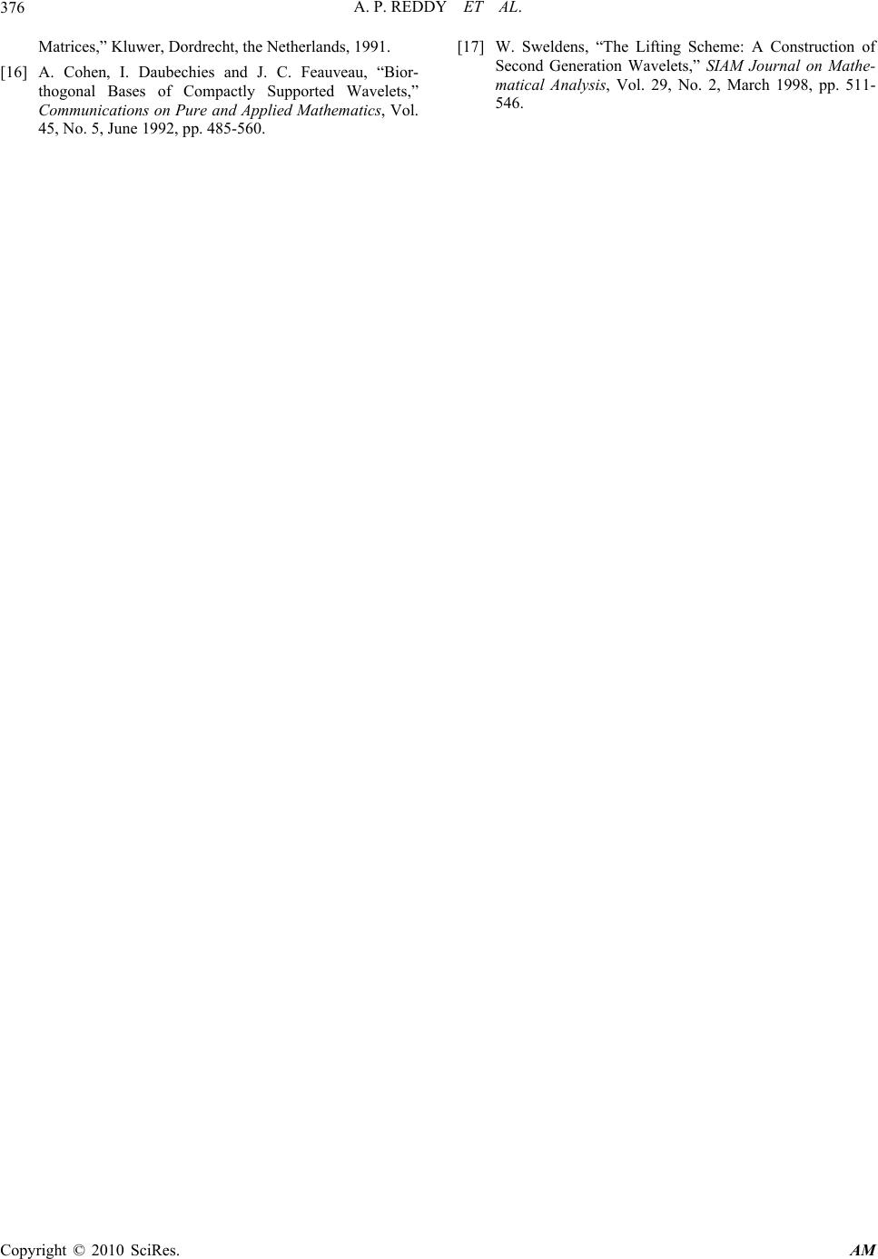

A. P. REDDY ET AL. 376
Matrices,” Kluwer, Dordrecht, the Netherlands, 1991.
[16] A. Cohen, I. Daubechies and J. C. Feauveau, “Bior-
thogonal Bases of Compactly Supported Wavelets,”
Communications on Pure and Applied Mathematics, Vol.
45, No. 5, June 1992, pp. 485-560.
[17] W. Sweldens, “The Lifting Scheme: A Construction of
Second Generation Wavelets,” SIAM Journal on Mathe-
matical Analysis, Vol. 29, No. 2, March 1998, pp. 511-
546.