Applied Mathematics, 2010, 1, 335-343
doi:10.4236/am.2010.15044 Published Online November 2010 (http://www.SciRP.org/journal/am)
335
Some Models of Reproducing Graphs: III Game Based
Reproduction
Richard Southwell, Chris Cannings
School of Mathematics and Statistics, University of Sheffield, Sheffield, United Kingdom
Received July 29, 2010; revised September 16, 2010; accepted September 18, 2010
Abstract
Many real world networks change over time. This may arise due to individuals joining or leaving the net-
work or due to links forming or being broken. These events may arise because of interactions between the
vertices which occasion payoffs which subsequently determine the fate of the vertices, due to ageing or
crowding, or perhaps due to isolation. Such phenomena result in a dynamical system which may lead to
complex behaviours, to selfreplication, to chaotic or regular patterns, or to emergent phenomena from local
interactions. They hopefully give insight to the nature of the real-world phenomena which the network, and
its dynamics, may approximate. To a large extent the models considered here are motivated by biological
and social phenomena, where the vertices may be genes, proteins, genomes or organisms, and the links in-
teractions of various kinds. In this, the third paper of a series, we consider the vertices to be players of some
game. Offspring inherit their parent’s strategies and vertices which behave poorly in games with their
neighbours get destroyed. The process is analogous to the way different kinds of animals reproduce whilst
unfit animals die. Some game based systems are analytically tractable, others are highly complex-causing
small initial structures to grow and break into large collections of self replicating structures.
Keywords: Reproduction, Graph, Network, Game, Replication
1. Introduction
With the growth of the internet and digital economy, it is
becoming increasingly important to understand how the
way individuals interact relates to the structure of the
network connecting them. This is also important in bio-
logy where the spatial distribution of individuals has a
profound effect upon the evolution of the ecosystem.
Evolutionary games on networks have recently be-
come a popular way to study these issues. Often one
considers a static network within which vertices (which
are thought of as players) adapt their strategies over time
as they play games with their neighbours [1-3]. A ques-
tion which is often asked about these systems is how
does the topology of the network affect the behaviour of
the players?
It is worth noting, however, that many real world
networks, such as the internet, ecosystems, economies
and social networks, are highly dynamic and often
change in response to strategic decisions of vertices. To
study this issue we propose a class of models where
networks grow in a way that depends upon the strategic
interactions of the vertices within. Looking at these
systems we can ask a different question how does the
behaviour of the players affect the topology of the
network?
In [4] we introduced eight reproducing graph models
within which graphs grow because their vertices re-
produce. In [5] we extended these models to include the
idea that vertices die of old age. In this paper (which is
an elaboration of [6]) we extend these models in a
different direction by incorporating game theory.
Our models are inspired by the way that animal social
networks develop as individuals reproduce in the sum-
mer whilst weak individuals perish in the winter. In our
models graphs change because the vertices (which have
different strategies) reproduce asexually. The offspring
are born with the parent’s strategy and link up to their
surroundings in similar way to their parents. This is
rather like the way newborn animals inherit their parent’s
genes and environment. The vertices play games and
gain payoffs as they interact with each another. Vertices

R. SOUTHWELL ET AL. 336
which perform poorly get destroyed whilst successful
vertices survive to further reproduce.
The systems we study can generate a rich variety of
different types of dynamics. Some cases are tractable and
we can derive powerful results which allow us to predict
the evolution of structures under a variety of games.
Other systems can generate remarkably complex dyna-
mics involving self replicating structures. Some very
simple games cause small initial structures to grow and
break up into diverse collections of self replicating
structures. Adaptive graph models that promote self
replication have been studied before in [7], where the
authors use genetic algorithms to find models that induce
self replication. The difference between this work and
ours is that our models were not explicitly designed to
promote self replication. This fascinating behaviour
arose unexpectedly as a result of our biologically
inspired rules.
2. The Models
In each of our models a graph =( ,)
ttt
GVE evolves
over discrete time steps t. We think of each vertex
t
vV as a player which employs some strategy
() {1,2,}vk

. The game which the vertices play is
specified by a kk payoff matrix
M
so that ,ij
M
is
the payoff which an employer of the ith strategy
receives against an employer of the jth. To obtain the
graph at the next time step we update t
G according to a
two stage process.
In the first (reproduction) stage we simultaneously
give each vertex an offspring vertex - which is born with
its parent’s strategy. The way these newborn vertices are
connected up depends upon which of the eight
reproduction mechanism from [4] we choose to use.
In model 0 offspring have no connections.
In model 1 offspring are connected to their parent’s
neighbours.
In model 2 offspring are connected to their parents.
In model 3 offspring are connected to their parents
and their parent’s neighbours.
In model 4 offspring are connected to the offspring
of their parent’s neighbours.
In model 5 offspring are connected to their parents
and the offspring of their parent’s neighbours.
In model 6 offspring are connected to their parent’s
neighbours and their parent’s neighbour’s offspring.
In model 7 offspring are connected to their parents,
their parent’s neighbours and the offspring of their
parent’s neighbours.
We let ()
m
RG denote the graph obtained by per-
forming the reproduction stage upon G according to
the thm reproduction model.
After the reproduction stage we perform the killing
stage. In this stage we remove every vertex which scores
a total payoff below some pre-specified `fitness’ threshold

. The total payoff (), ()
()
()= vu
uNev
fit vM


 of a
vertex v is the total score it gets when it plays a game
with each member of its neighbourhood ()Ne v.
Sometimes we shall refer to the total payoff of a vertex
as its fitness. We let ()CG

denote the graph obtained
by applying the killing stage to a graph G using fitness
threshold

.
Our update operator U is defined so that ()=UG
(())
m
CRG

is the graph obtained by performing the
reproduction stage followed by the killing stage. The
graph obtained by updating t G is 1=()
tt
GUG
. In this
paper we shall study how the structure 0 =()
t
t
GUG
changes over time steps t for different choices of initial
graph 0
G, game
M
, reproduction model m and
fitness threshold

.
The dynamics under reproduction models 70,2,4,5,6,
and 8 are quite tractable. Later we shall derive
powerful results which allow one to predict many
features of the evolution of arbitrary games under these
systems. Highly complex self replicative dynamics occur
when reproduction models 1 or 3 are employed. In [6]
we explore this phenomenon when =1m. We shall
begin this paper with a discussion of self replication
when =3m.
3. Self Replication When 3m=
The =3m growth model is the most complicated. Even
under pure reproduction [4] (where vertices are immortal)
this model generates a complex structure with an
interesting degree distribution [8]. When we incorporate
game theory we almost immediately see complex be-
haviour.
3.1. A One Strategy Case: Degree Capped
Reproduction
Even when we investigate the dynamics of one strategy
games we find a system of immense complexity, which
we call degree capped reproduction. In this case
=Q


, for some positive integer Q, and we begin
with a graph 0
G where all vertices employ a strategy
that scores a payoff of −1 against itself. Updating a graph
t
G under the degree capped reproduction model
consists of performing two stages.
Stage 1, Reproduce: simultaneously give every vertex
of t G an offspring vertex which is connected to its
parent and its parent’s neighbours.
Stage 2, Kill: remove every vertex of degree greater
than Q.

R. SOUTHWELL ET AL. 337
Under degree capped reproduction graphs tend to
grow and break into other graphs. Phase diagrams
represent how connected structures produce one another
using arrows. The arrows pointing out of a graph point
towards the connected graphs produced by updating it.
The numbers on the arrows correspond to the numbers of
such graphs produced.
When we evolve an isolated vertex under degree
capped reproduction with =4Q we get the dynamics
depicted in Figure 1. The structure grows up over the
first two updates and then breaks into four more isolated
vertices. These vertices continue to replicate in a similar
way.
The way the isolated vertex evolves when =5Q is
considerably more elaborate Figure 2. In this case the
structure grows over the first four updates to become a
square structure with four ‘arms’. This structure breaks
into four smaller structures which replicate themselves
and other self replicating structres. Eventually more
isolated vertices are generated and one is left with a soup
of eleven different kinds of self replicating graphs.
As Q increases the self replicative behaviour be-
comes increasingly intricate. Figure 3 shows the self
replicative habits of the 13 different graphs that grow
from an isolated vertex when =7Q.
Increasing Q further causes an immense increase in
complexity. When =10,Q the isolated vertex even-
tually generates an ecosystem of 121 different kinds of
self replicating structures. These structures produce
copies of one another according to a large phase diagram
similar to Figure 7. This behaviour is incredibly
complicated, many of the structures produced have
hundreds of vertices. Figure 4 shows an example.
There is much more to study about degree capped
reproduction. We conjecture that every finite initial
condition generates a bounded number of different self
replicating structures under finite Q. A method to prove
this conjecture or identify the self replicating structures
would be highly desirable. However the rapid increase in
complexity with Q makes it doubtful that such a
method can be found.
Degree capped reproduction can be thought of as a toy
model for the way an animal social network changes
over time. Consider a set of reproducing individuals
which share some vital resource, like food. When new
offspring are born they will share resources with their
parents and their parent’s associates. When an individual
shares its resources with too many other individuals it
starves and dies.
Figure 1. A phase diagram showing how the different
structures that grow from an isolated vertex generate each
other when 4Q= .
Figure 2. A phase diagram showing how the different structures that grow from an isolated vertex generate each other when
5Q= .

R. SOUTHWELL ET AL. 338
Figure 3. A phase diagram showing how the different structures that grow from an isolated vertex generate each other when
7Q= .
Figure 4. One of the 121 self replicating structures that get produced when one evolves an isolated vertex with 10Q= . This
graph has 292 vertices.
It is remarkable how these simple biologically inspired
rules can give rise to such a diverse collection of self
replicating structures. It suggests that complex self
replicating structures, like life, do not have to be the
result of complex rules. Self replication has been
achieved by other decentralised systems, like cellular
automata, but in our systems we see self replicating
structures that can diversify their forms. If we extended
our models to include some external forces which
destroy vertices based upon local topology it seems

R. SOUTHWELL ET AL. 339
likely our structures will ‘evolve’ towards self replicating
forms that suit their external environment.
3.2. An Example with Two Strategies
Many other types of behaviour can be produced when
reproduction model 3 is used with other games.
Consider, for example, the case where =12

 and the
game is specified by the payoff matrix
32
05





When we run this system, starting with the graph
shown in Figure 5, we see a large structure grow up that
contains employers of both strategies. The large structure
seems to grow relentlessly whilst throwing off mono
strategy fragments that self replicate in accordance with
degree capped reproduction.
This coexistence of self replicating structures on
different scales also occurs in biological processes. As
large organisms grow they house many micro organisms
which compete and reproduce. Occasionally these micro
organisms may leave the body of their host to self
replicate elsewhere.
There is much more to study about the dynamics of
games when =3m. It appears as though when 0


the dynamics are relatively constrained. In cases like this
structures seem to either die away or reach a regime of
unrelenting growth without structural disconnections.
We have made a brief exploration of game dynamics
when <0

but many mysteries remain. Are there any
games which cause the number of vertices to fluctuate
chaotically over time? Does there exist a game which
generates a computationally universal system (in that
arbitrary computations can be emulated by evolving
appropriate initial conditions)?
4. The Dynamics When 1m=
Model 1 is the other growth mechanism that can
produce highly complex behaviour. A vertex v will
survive the U update when =1m if and only if
() 2 fit v

 whilst v‘s offspring will be present after the
U update if and only if ()fit v

.
The complexity of ()
t
UG’s dynamics depends
largely upon the sign of the fitness threshold

. When
=0

the dynamics are relatively easy to describe,
structures either grow forever or fizzle away to nothing.
When >0

it seems (although we cannot prove) that
connected structures either grow forever, fizzle away, or
become fixed. When <0

dynamics of enormous
complexity can ensue.
Figure 5. The evolution of an example structure when

12τ= and the game is as defined in Subsection 3.2. The
arrows denote update operations (which may lead to
structures breaking into pieces). Employers of strategies 1
and 2 are represented by white and black vertices res-
pectively.
4.1. The Case When 0τ=
The easiest case is when 0=

; in this case we have
).)((=))((=)(0110 GCRGRCGU  (1)
where
f
g denotes the composition of functions
f
and
g
.
Swapping round the order of killing and reproduction
allows us to gain the expression
011 0
()=( )()=()().
tttt
UGCRGRCG (2)
So in other words ()
t
UG is the graph obtained by
taking G and applying the killing operator to it t

R. SOUTHWELL ET AL. 340
times and then applying the reproduction operator to the
resulting graph t times.
A vertex v in G will reproduce forever under t U
if and only if it does not get removed by the 0 C

operation. This means every finite graph will either die
out or reach a regime of unbounded growth.
4.2. The Case When >0τ
When 0>

it seems that the long term behaviour of
)(GU t is again quite restricted. We conjecture that any
graph G will evolve under t
U towards either
destruction, unbounded growth or some mixture of fixed
subgraphs and subgraphs that grow forever (in that none
of their descendants ever die). Computer simulations are
our main reason for believing this however we can
demonstrate some restrictions when
M
is non-nega-
tive.
When 0>

and
M
has no negative entries then
for any initial graph G we will have
1
22
11
2
() ()().
tt
ttt t
RCGUGRC CCG



 (3)
Thus vertices of G that get removed by the
12
22
tt
CC C




(4)
operation, as t, will certainly not enter a regime of
unrestricted reproduction. On the other hand vertices that
survive the t C

operation, as t, will surely
reproduce forever. Somewhere between these two
extremes are vertices that become infertile and immortal
(i.e. static). When all vertices are static the graph will be
fixed under the U update; this occurs when each vertex
has a fitness in ,
2






.
4.3. The case when 0τ<
When <0

exotic dynamics can occur. In addition to
the null, fixed and unbounded growth behaviour types
that we found before, when <0

, we encounter self
replicative dynamics similar to those discussed in section
3 ([6] is largely devoted to the study of this phenomena).
In [6] we made an extensive investigate of the dynamics
of degree capped reproduction when individuals
reproduce according to the =1m model (i.e. when
offspring are not connected to their parents).
The dynamics of degree capped reproduction when
=1m are similar to those when =3m. When Q is
small structures tend to generate a reasonably small
collection of self replicating structures. Figure 6 shows
the structures that get generated when one evolves a
single edge under this system with =4Q.
Again as one increases Q one sees a dramatic
increase in the complexity of the self replicative
processes. Figure 7 shows a phase diagram which
illustrates how the 210 self replicating structures that
get made by evolving a single edge produce each other.
In [6] we demonstrate how this self replicative
behaviour persists when one adds a degree of ran-
domness into the update procedure. In this paper we also
describe many two strategy games that can promote self
replication.
5. The Dynamics When 2m=
The dynamics of ()
t
UG when =2m are very similar
to dynamics of reproduction model 2 in the age capped
systems [5]. Offspring are born only connected to their
parent and so repeated updates cause tree structures to
sprout out of the initial graph structure (which may itself
disintegrate). The fundamental form of the tree that will
grow out of a vertex employing a given strategy is just
Figure 6. A phase diagram showing the self replicating
structures which emerge from evolving a single edge when
=4Q and =3m.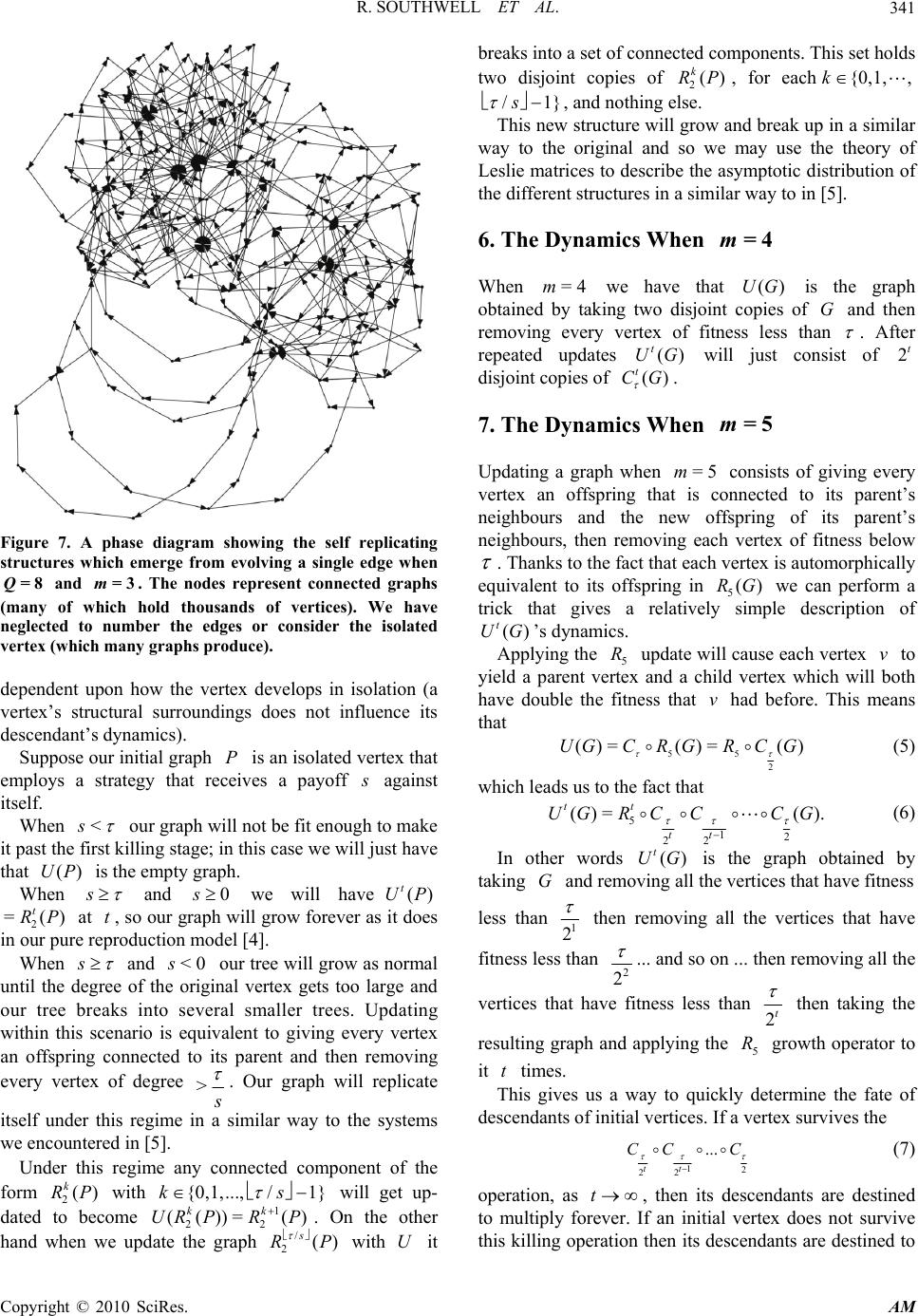

R. SOUTHWELL ET AL. 341
Figure 7. A phase diagram showing the self replicating
structures which emerge from evolving a single edge when
=8Q and =3m. The nodes represent connected graphs
(many of which hold thousands of vertices). We have
neglected to number the edges or consider the isolated
vertex (which many graphs produce).
dependent upon how the vertex develops in isolation (a
vertex’s structural surroundings does not influence its
descendant’s dynamics).
Suppose our initial graph P is an isolated vertex that
employs a strategy that receives a payoff
s
against
itself.
When <
s

our graph will not be fit enough to make
it past the first killing stage; in this case we will just have
that ()UP is the empty graph.
When s

 and 0s we will have()
t
UP
2
=()
t
RP at
t
, so our graph will grow forever as it does
in our pure reproduction model [4].
When s

 and <0s our tree will grow as normal
until the degree of the original vertex gets too large and
our tree breaks into several smaller trees. Updating
within this scenario is equivalent to giving every vertex
an offspring connected to its parent and then removing
every vertex of degree >
s

. Our graph will replicate
itself under this regime in a similar way to the systems
we encountered in [5].
Under this regime any connected component of the
form 2()
k
RP with {0,1,..., /1}ks   will get up-
dated to become 1
22
(())= ()
kk
UR PRP
. On the other
hand when we update the graph /
2()
s
RP
  with U it
breaks into a set of connected components. This set holds
two disjoint copies of 2()
k
RP
, for each{0,1, ,k


/1}s 

 , and nothing else.
This new structure will grow and break up in a similar
way to the original and so we may use the theory of
Leslie matrices to describe the asymptotic distribution of
the different structures in a similar way to in [5].
6. The Dynamics When 4m=
When =4m we have that ()UG is the graph
obtained by taking two disjoint copies of G and then
removing every vertex of fitness less than

. After
repeated updates ()
t
UG will just consist of 2t
disjoint copies of ()
t
CG

.
7. The Dynamics When 5m=
Updating a graph when =5m consists of giving every
vertex an offspring that is connected to its parent’s
neighbours and the new offspring of its parent’s
neighbours, then removing each vertex of fitness below

. Thanks to the fact that each vertex is automorphically
equivalent to its offspring in 5()RG we can perform a
trick that gives a relatively simple description of
()
t
UG ’s dynamics.
Applying the 5
R update will cause each vertex v to
yield a parent vertex and a child vertex which will both
have double the fitness that v had before. This means
that
)(=)(=)(
2
55 GCRGRCGU 
 (5)
which leads us to the fact that
5
12
22
()= ().
tt
tt
UGR CCCG
 

  (6)
In other words ()
t
UG is the graph obtained by
taking G and removing all the vertices that have fitness
less than 1
2

then removing all the vertices that have
fitness less than 2
2

... and so on ... then removing all the
vertices that have fitness less than 2t

then taking the
resulting graph and applying the 5 R growth operator to
it t times.
This gives us a way to quickly determine the fate of
descendants of initial vertices. If a vertex survives the
12
22
...
tt
CC C



 (7)
operation, as t, then its descendants are destined
to multiply forever. If an initial vertex does not survive
this killing operation then its descendants are destined to

R. SOUTHWELL ET AL. 342
eventually die out. This allows us to predict the dyna-
mics of our models with much less effort. It also implies
that the rich self replicative dynamics observed when
=1m and =3m cannot occur under this model.
8. The Dynamics When 6m=
Updating a graph G under the =6m model consists
of making an ‘offspring copy’ of G, linking each vertex
with its offspring in the offspring copy, and then
removing every vertex that has fitness below

. The
symmetry between parents and their offspring allows us
to do a similar trick to that used to simplify the =5m
case.
Let ,n C

be defined such that for any strategy
attributed graph G we have that ,()
n
CG

is the graph
obtained by taking G and removing each vertex v
such that (), () () .<
vv
fitvn M


.
After the 6 R update both the offspring and the
surviving parent will have the fitness of their original
vertex plus the score that their strategy gets against itself
(the effect of the ‘umbilical connection’ between parent
and offspring). This means
0,661,
()=()= ()UGCRGRCG


(8)
from which it follows that
6 ,1,1,
()=().
tt
tt
UGR CCCG
  
  (9)
This means that again one can say in advance whether
the descendants of initial vertices will die out or multiply
forever.
9. The Dynamics When 7m=
Updating a graph with =7m consists of giving every
vertex an offspring with the same strategy that is
connected to its parent, its parent’s neighbours and the
new offspring of its parent’s neighbours, and then
removing every vertex of fitness less than

. Again
symmetry allows us to do a trick that gives us a simpler
view of the dynamics.
For any vertex v of fitness ()
f
it v in G both v
and v’s offspring within 7()RG will have fitness
(), ()
2.()vv fit vM

. Let
()=2
y
hxx y (10)
and let
*
,() r
CG

(11)
be the graph obtained by taking G and removing every
vertex such that
(), ()
(())<.
r
Mvv
hfit v


(12)
In this case we will have that
**
0,771,
()=()= ()UGCR GRCG

 (13)
which means that
** *
7, 1,1,
()=()
tt
tt
UGR CCCG
  
  (14)
so again we can determine the fate of our initial vertices
descendants without explicitly running the system.
10. Conclusions
In this paper we have investigated many features of game
theory based reproducing graph models. Many kinds of
behaviour can be generated and there are many
perspectives through which one may view these systems.
From an evolutionary game theory standpoint these
systems are interesting because they provide a (possibly
analytic) method to investigate how the outcome of
games effects the formation of communities. To
investigate this it would be useful to compare the
dynamics of our graphs with the behaviour of other
systems based upon game theory.
From the perspective of theoretical biology and
artificial life these systems are interesting because they
can demonstrate rich self replicative behaviour. The
existence of these systems begs the question of what
other adaptive graph models can do. Finding other
systems with similar behaviour might be useful for
modeling systems in biology and inventing nano-
technology.
From the perspective of complex systems research
these systems are interesting because they can generate
highly complex behaviour from simple initial conditions.
An interesting question from this perspective is just how
complicated our systems are. Is there a simple formula to
describe the dynamics of graphs under degree capped
reproduction? Are features of their dynamics formally
undecidable?
Taking a more practical perspective one might ask
what real world applications these systems may have.
Using game theory to reward or punish graphs for
growing in particular ways could be an interesting way
of designing networks for specific purposes. It would be
interesting to see if one could use systems similar to
those we have discussed for design of communication
networks or self repairing structures.
11. Acknowledgements
The authors gratefully acknowledge support from the
EPSRC (Grant EP/D003105/1) and helpful input from Dr
Jonathan Jordan, Dr Seth Bullock and others in the

R. SOUTHWELL ET AL. 343
Amorph Research Project (www.amorph.group.shef.ac.
uk).
12. References
[1] M. Nowak and R. May, “Evolutionary Games and Spatial
Chaos,” Nature, Vol. 359, No. 6398, 1992, pp. 826-829.
[2] R. Southwell and C. Cannings, “Best Response Games on
Regular Graphs,” Under Review, 2010.
[3] F. Santos, J. Pacheco and T. Lenaerts, “Evolutionary
Dynamics of Social Dilemmas in Structured Heteroge-
neous Populations,” Proceedings of the National Acad-
emy of Sciences of the United States of America, Iowa,
Vol. 103, 2006, pp. 3490-3494.
[4] R. Southwell and C. Cannings, “Some Models of Repro-
ducing Graphs: I Pure Reproduction,” Applied Mathe-
matics, Vol. 1, No. 3, 2010, pp. 137-145.
[5] R. Southwell and C. Cannings, “Some Models of Repro-
ducing Graphs: II Age Capped Vertices,” Applied Mathe-
matics, Vol. 1, No. 4, 2010, pp. 251-259.
[6] R. Southwell and C. Cannings, “Games on Graphs that
Grow Deterministically,” Proceedings of the 1st Interna-
tional Conference on Game Theory for Networks
(GameNets), Istanbul, 13-15 May 2009.
[7] H. Tomita, H. Kurokawa and S. Murata, “Automatic
Generation of Self-Replicating Patterns in Graph Auto-
mata,” International Journal of Bifurcation and Chaos,
Vol. 16, No. 4, 2006, pp. 1011-1018.
[8] J. Jordan and R. Southwell, “Further Properties of Re-
producing Graphs,” Under Review, 2010.