Journal of Global Positioning Systems (2005)
Vol. 4, No. 1-2: 230-239
Troposphere Modeling in a Regional GPS Network
S. Skone and V. Hoyle
Department of Geomatics Engineering, University of Calgary, 2500 University Dr. N.W., T2N 1N4 Calgary, Canada
e-mail: [e-mail] Tel: + 01-403-220-7589; Fax: [phone]
Received: 16 November 2004 / Accepted: 12 July 2005
Abstract. By using a regional network of Global
Positioning System (GPS) reference stations, it is
possible to recover estimates of the slant wet delay
(SWD) to all GPS satellites in view. SWD observations
can then be used to model the vertical and horizontal
structure of water vapor over a local area, using a
tomographic approach. The University of Calgary
currently operates a regional GPS real-time network of 14
sites in southern Alberta. This network provides an
excellent opportunity to study severe weather conditions
(e.g. thunderstorms, hail, and tornados) which develop in
the foothills of the Rockies near Calgary. In this paper, a
4-D tomographic water vapor model is tested using the
regional GPS network. A field campaign was conducted
during July 2003 to derive an extensive set of truth data
from radiosonde soundings. Accuracies of tomographic
water vapor retrieval techniques are evaluated for 1)
using only ground-based GPS input, and 2) using a
ground-based GPS solution augmented with vertical wet
refractivity profiles derived from radiosondes released
within the GPS network. Zenith wet delays (ZWD) are
computed for both cases, by integrating through the 4-D
tomography predictions, and these values are compared
with truth ZWD derived from independent radiosonde
measurements. Results indicate that ZWD may be
modeled with accuracies at the sub-centimeter level using
a ground-based GPS network augmented with vertical
profile information. This represents an improvement
over the GPS-only approach.
Key words: troposphere, water vapor, tomography, GPS,
positioning, atmospheric errors Ionosphere, WADGPS,
WAAS
1 Introduction
GPS range observations are derived under the assumption
that GPS signals travel at the speed of light (or,
equivalently, the index of refraction is equal to one) along
the satellite-receiver signal path. For GPS orbits of
approximately 20,000 km altitude, the signal must travel
through the Earth’s ionosphere and neutral atmosphere.
In these regions indices of refraction can differ
significantly from assumptions, such that range errors
arise from signal propagation through the Earth’s
atmosphere. The range errors induced by the ionosphere
are dispersive and 99% of the ionospheric effect may be
removed using dual frequency GPS observations
(Brunner and Gu, 1991).
Range errors associated with propagation through the
neutral atmosphere can be classified as a hydrostatic
component and a wet delay. The total delay s∆ is related
to the neutral refractivity N as follows:
∫
=∆
path 6ds
10
N
s (1)
where N may be expressed as (cf. Ware et al., 1997)
wh
wet
2
5
chydrostati
NN
T
e
1073.3
T
P
6.77N +=×+=


(2)
The variable P represents air pressure in millibars, T is
the temperature in degrees Kelvin and e is the partial
pressure of water vapor in millibars. Th e va riables Nh and
NW represent the hydrostatic and wet refractivities,
respectively. The total tropospheric range delay (Equation
1) can therefore be expressed as the sum of both wet and
hydrostatic components:
SWDSHDs
+
=
∆
(3)
where SHD and SWD refer to the slant hydrostatic and
slant wet delays, respectively, along the signal path.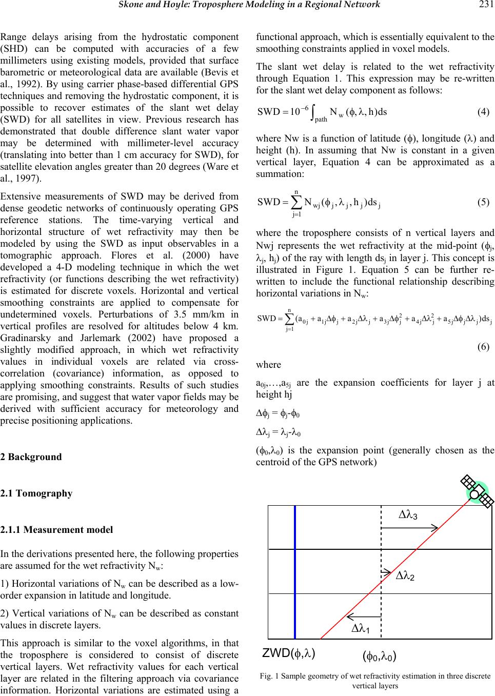

Skone and Hoyle: Troposphere Modeling in a Regional Network 231
Range delays arising from the hydrostatic component
(SHD) can be computed with accuracies of a few
millimeters using existing models, provided that surface
barometric or meteorological data are available (Bevis et
al., 1992). By using carrier phase-based differential GPS
techniques and removing the hydrostatic component, it is
possible to recover estimates of the slant wet delay
(SWD) for all satellites in view. Previous research has
demonstrated that double difference slant water vapor
may be determined with millimeter-level accuracy
(translating into better than 1 cm accuracy for SWD), for
satellite elevation angles greater than 20 degrees (Ware et
al., 1997).
Extensive measurements of SWD may be derived from
dense geodetic networks of continuously operating GPS
reference stations. The time-varying vertical and
horizontal structure of wet refractivity may then be
modeled by using the SWD as input observables in a
tomographic approach. Flores et al. (2000) have
developed a 4-D modeling technique in which the wet
refractivity (or functions describing the wet refractivity)
is estimated for discrete voxels. Horizontal and vertical
smoothing constraints are applied to compensate for
undetermined voxels. Perturbations of 3.5 mm/km in
vertical profiles are resolved for altitudes below 4 km.
Gradinarsky and Jarlemark (2002) have proposed a
slightly modified approach, in which wet refractivity
values in individual voxels are related via cross-
correlation (covariance) information, as opposed to
applying smoothing constraints. Results of such studies
are promising, and suggest that water vapor fields may be
derived with sufficient accuracy for meteorology and
precise positioning applications.
2 Background
2.1 Tomography
2.1.1 Measurement model
In the derivations presented here, the following properties
are assumed for the wet refractivity Nw:
1) Horizontal variations of Nw can be described as a low-
order expansion in latitude and longitude.
2) Vertical variations of Nw can be described as constant
values in discrete layers.
This approach is similar to the voxel algorithms, in that
the troposphere is considered to consist of discrete
vertical layers. Wet refractivity values for each vertical
layer are related in the filtering approach via covariance
information. Horizontal variations are estimated using a
functional approach, which is essentially equivalent to the
smoothing constraints applied in voxel models.
The slant wet delay is related to the wet refractivity
through Equation 1. This expression may be re-written
for the slant wet delay component as fo llows:
∫λφ= −
path w
6ds)h,,(N10SWD (4)
where Nw is a function of latitude (φ), longitude (λ) and
height (h). In assuming that Nw is constant in a given
vertical layer, Equation 4 can be approximated as a
summation:
jjjj
n
1j wj ds)h,,(NSWD λφ= ∑ =
(5)
where the troposphere consists of n vertical layers and
Nwj represents the wet refractivity at the mid-point (φj,
λj, hj) of the ray with leng th dsj in layer j. This concept is
illustrated in Figure 1. Equation 5 can be further re-
written to include the functional relationship describing
horizontal variations in Nw:
jjjj5
2
jj4
2
jj3jj2j
n
1j j1j0ds)aaaaaa(SWD λ∆φ∆+λ∆+φ∆+λ∆+φ∆+= ∑ =
(6)
where
a0j,…,a5j are the expansion coefficients for layer j at
height hj
∆φj = φj-φ0
∆λj = λj-λ0
(φ0,λ0) is the expansion point (generally chosen as the
centroid of the GPS net wo rk )
Fig. 1 Sample geom etry of wet refractivity estimation in three discrete
vertical layers
(
φ
0,λ0
)
∆λ3
∆λ2
∆
λ
1
ZWD
(
φ
,
λ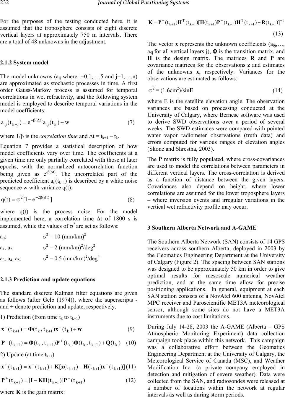
)

232 Journal of Global Positioning Systems
For the purposes of the testing conducted here, it is
assumed that the troposphere consists of eight discrete
vertical layers at approximately 750 m intervals. There
are a total of 48 unknowns in the adjustment.
2.1.2 System model
The model unknowns (aij where i=0,1,…,5 and j=1,…,n)
are approximated as stochastic processes in time. A first
order Gauss-Markov process is assumed for temporal
correlations in wet refractivity, and the following system
model is employed to describe temporal variations in the
model coefficients:
w)t(ae)t(a kij
)t(
1kij += ∆β−
+ (7)
where 1/β is the correlation time and ∆t = tk+1 – tk.
Equation 7 provides a statistical description of how
model coefficients vary over time. The coefficients at a
given time are only partially correlated with those at later
epochs, with the normalized autocorrelation function
being given as e-β(∆t). The uncorrelated part of the
predicted co efficient aij(tk+1) is described by a white noise
sequence w with variance q(t):
]e1[)t(q )t(22 ∆β− −σ= (8)
where q(t) is the process noise. For the model
implemented here, a correlation time ∆t of 1800 s is
assumed, while the values of σ2 are set as follows:
a0: σ2 = 10 (mm/km)2
a1, a2: σ2 = 2 (mm/km )2/deg2
a3, a4, a5: σ2 = 0.5 (mm/km )2/deg4
2.1.3 Prediction and update equations
The standard discrete Kalman filter equations are given
as follows (after Gelb (1974)), where the superscripts -
and + denote prediction and update, respectively.
1) Prediction (from time tk to tk+1)
wxΦx+= +
++
−)t()t,t()t( k1kk1k (9)
)t()t,t()t()t,t()t( k1kkk1kk1kQΦPΦP+= +
+
++
− (10)
2) Update (at time tk+1)
)]t()t()t([)t()t( 1k1k1k1k1k +
−
+++
−
+
+−+= xHzKxx (11)
)t()]t([)t( 1k1k1k +
−
++
+−= PKHIP (12)
where K is the gain matrix:
1
1k1k
T
1k1k1k
T
1k)]t()t()t()t()[t()t( − +++
−
+++
−+= RHPHHPK
(13)
The vector x represents the unknown coefficients (a0j,…,
a5j for all vertical layers j), Φ is the transition matrix, and
H is the design matrix. The matrices R and P are
covariance matrices for the observations z and estimates
of the unknowns x, respectively. Variances for the
observations are estimated as follows:
2
σ= (1.6cm2)/sinE (14)
where E is the satellite elevation angle. The observation
variances are based on processing conducted at the
University of Calgary, where Bernese software was used
to derive SWD observations over a period of several
weeks. The SWD estimates were compared with pointed
water vapor radiometer observations (truth data) and
errors computed for various ranges of elevation angles
(Skone and Shrestha, 2003).
The P matrix is fully populated, where cross-covariances
are used to model the correlations between parameters in
different vertical layers. The cross-correlation is derived
as a function of distance between the given layers.
Covariances also depend on height, where lower
correlations are assumed for the lower troposphere layers
– where inversion events and irregular variations in the
vertical wet refractivity profile may occur.
3 Southern Alberta Network and A-GAME
The Southern Alberta Network (SAN) consists of 14 GPS
receivers across southern Alberta, deployed in 2003 by
the Geomatics Engineering Department at the University
of Calgary (Figure 2). The spacing between SAN stations
was designed to be approximately 50 km in order to give
optimal results for mesoscale numerical weather
prediction, and at the same time allow for precise
positioning applications. In general, equipment at each
SAN station consists of a NovAtel 600 antenn a, NovAtel
MPC receiver and Paroscientific MET3A meteorological
sensor, although some sites do not have a MET3A
instruments due to cost limitations.
During July 14-28, 2003 the A-GAME (Alberta – GPS
Atmospheric Monitoring Experiment) data collection
campaign took place within this network. This campaign
was a collaborative effort between the Geomatics
Engineering Department at the University of Calgary, the
Meteorological Service of Canada (MSC), and Weather
Modification Inc. (a private company employed in
detection and mitigation of severe weather). Data were
collected from the SAN, and radiosondes were released at
a number of locations within the network at regular
intervals as well as during storm periods.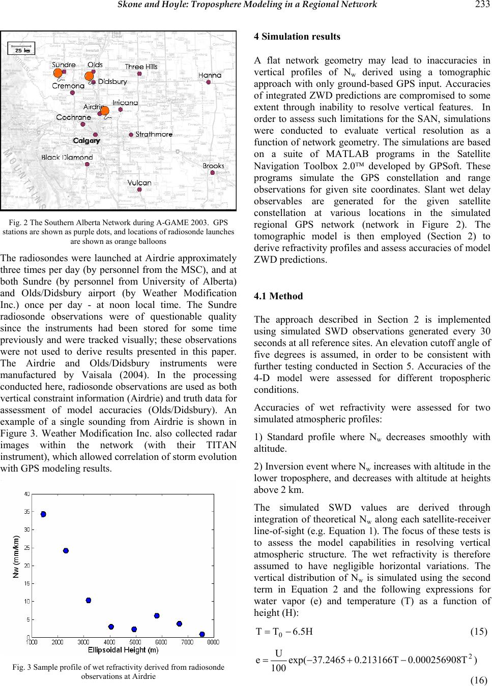

Skone and Hoyle: Troposphere Modeling in a Regional Network 233
Fig. 2 The Southern Alberta Network during A-GAME 2003. GPS
stations are shown as purple dots, and locations of radio sonde launches
are shown as orange balloons
The radiosondes were launched at Airdrie approximately
three times per day (by personnel from the MSC), and at
both Sundre (by personnel from University of Alberta)
and Olds/Didsbury airport (by Weather Modification
Inc.) once per day - at noon local time. The Sundre
radiosonde observations were of questionable quality
since the instruments had been stored for some time
previously and were tracked visually; these observations
were not used to derive results presented in this paper.
The Airdrie and Olds/Didsbury instruments were
manufactured by Vaisala (2004). In the processing
conducted here, radiosonde observations are used as both
vertical constraint information (Airdrie) and truth data for
assessment of model accuracies (Olds/Didsbury). An
example of a single sounding from Airdrie is shown in
Figure 3. Weather Modification Inc. also collected radar
images within the network (with their TITAN
instrument), which allowed correlation of storm evolution
with GPS modeling results.
Fig. 3 Sample profile of wet r efractivity derived from radiosonde
observations at Airdrie
4 Simulation results
A flat network geometry may lead to inaccuracies in
vertical profiles of Nw derived using a tomographic
approach with only ground-based GPS input. Accuracies
of integrated ZWD predictions are compromised to some
extent through inability to resolve vertical features. In
order to assess such limitations for the SAN, simulations
were conducted to evaluate vertical resolution as a
function of network geometry. The simulations are based
on a suite of MATLAB programs in the Satellite
Navigation Toolbox 2.0™ developed by GPSoft. These
programs simulate the GPS constellation and range
observations for given site coordinates. Slant wet delay
observables are generated for the given satellite
constellation at various locations in the simulated
regional GPS network (network in Figure 2). The
tomographic model is then employed (Section 2) to
derive refractivity profiles and assess accuracies of model
ZWD predictions.
4.1 Method
The approach described in Section 2 is implemented
using simulated SWD observations generated every 30
seconds at all reference sites. An elevation cutoff angle of
five degrees is assumed, in order to be consistent with
further testing conducted in Section 5. Accuracies of the
4-D model were assessed for different tropospheric
conditions.
Accuracies of wet refractivity were assessed for two
simulated atmospheric profiles:
1) Standard profile where Nw decreases smoothly with
altitude.
2) Inversion event where Nw increases with altitude in the
lower troposphere, and decreases with altitude at heights
above 2 km.
The simulated SWD values are derived through
integration of theoretical Nw along each satellite-receiver
line-of-sight (e.g. Equation 1). The focus of these tests is
to assess the model capabilities in resolving vertical
atmospheric structure. The wet refractivity is therefore
assumed to have negligible horizontal variations. The
vertical distribution of Nw is simulated using the second
term in Equation 2 and the following expressions for
water vapor (e) and temperature (T) as a function of
height (H):
H5.6TT 0
−
=
(15)
)T000256908.0T213166.02465.37exp(
100
U
e2 −+−=
(16)

234 Journal of Global Positioning Systems
where H is in kilometers, T is in Kelvin and and e is in
millibars. The variable U represents humidity (in percent)
and T0 is the temperature at sea level. For the simulations
presented here, U is assumed to be 50 percent and T0 is
293 °K. The simulated SWD observations have additional
random errors imposed as a function of elevation angle,
with magnitudes determined from Equation 14. The
inversion event is simulated by using Equations 15 and
16 for heights above 2 km, but imposing a positive
gradient (as a function of height) in the altitud e range 0-2
km.
4.2 Results
Figure 4 shows the wet refractivity estimates generated
by the model (after 30 minutes of processing) for the
standard profile. The truth data (the Nw profiles used to
generate the initial SWD observations) are also plotted
for comparison purposes. The Nw values predicted by the
model average through the truth profile – representing a
smoothed approximation of the vertical atmospheric
features. The Nw values are particularly poor at the lower
heights, where only one GPS site is located at an altitude
sufficiently low enough to observe the bottom
atmospheric layer.
Figure 5 shows the wet refractivity estimates for the
inversion event (after 30 minutes of processing) versus
the truth profile. The irregular inversion profile at lower
altitudes is not resolved in the tomography model, with
accuracies as poor as 10 mm/km at lower altitudes.
Similar to Figure 4, the model values represent a
smoothed average of the vertical atmospheric features
present above the GPS network. The ground-based GPS
observations alone would not allow resolution of
inversion profiles.
Results in Figures 4 and 5 demonstrate the impact of
network geometry - in particular, vertical station
separation within the network - in deriving wet
refractivity profiles using ground-based regional
networks. Vertical resolution is limited for a flat network
such as the SAN, with deficiencies in resolving irregular
profiles. For the case of an inversion event, the vertical
Nw values generated with a flat network represent only
the low-order variations – with an overall smoothing of
the true vertical profile.
Results in this section demonstrate that it is difficult to
resolve vertical Nw profiles for a flat network geometry,
using ground-based GPS data alone. Potential exists,
however, to exploit existing sources of vertical
information (such as radiosondes or climate models) to
constrain the vertical profiles in a tomography approach.
By achieving improved vertical resolution through
assimilation of such external data sources, it is anticipated
that improved ZWD predictions may be derived for GPS
users within the GPS network. This type of approach is
explored in the next section.
Fig. 4 Nw estimates (blue stars) versus truth (red curve) – standard Nw
profile
Fig. 5 Nw estimates (blue stars) versus truth (red curve) – inversion
event
5 Model results: A-GAME
This section shows model results derived using SAN
data, augmented with radiosonde observations, for the A-
GAME 2003 campaign. Results are derived for a number
of days representing various weather conditions. A brief
description of the processing approach and specific data
sets follows.
5.1 Estimation of SWD
Hourly estimates of total zenith delays were derived at
each receiver in the SAN, with the exception of Olds and
Didsbury (Figure 2), using Bernese version 4.2
(Hugentobler et al., 2001), with an ionosphere-free fixed

Skone and Hoyle: Troposphere Modeling in a Regional Network 235
approach using 30-second observations and an elevation
mask of five degrees. The hydrostatic component of the
total zenith delay was removed using the Saastamoinen
model for hydrostatic delay (cf. Bar-Server and Kroger,
1998):
)h00028.02cos00266.01(
P22765.0
DH−φ− = (17)
where DH is the hydrostatic delay in centimeters, P is the
pressure at the station in millibars, ϕ is the statio n latitu de
in degrees and h is the station height in kilometers. The
remaining zenith wet delay was then mapped to the
appropriate elevation angle using the Niell wet mapping
function (Niell, 1996). In this way, SWD observations
were derived for all satellites in view at each available
station within the SAN (Figure 2). These observation s are
used as input observables in the tomography model.
5.2 Radiosonde vertical NW constraints and truth data
As described in Section 3, radiosonde observations were
available at a number of SAN sites during the A-GAME
2003 campaign. These measurements can be used as
additional input ob servations for the tomographic model -
serving essentially as vertical profile constraints. The
addition of such high-resolution vertical information
allows improved 4-D modeling using the tomographic
approach, when combined with the SWD estimates from
GPS reference sites. For the tests conducted here, two
sets of radiosonde observations are used:
• Airdrie: vertical profiles of NW are derived and
assimilated into the tomogr aphy model.
• Olds/Disbury airport: vertical profiles of NW are
derived but excluded from the tomography
adjustment and instead used as independent truth
data – to assess model prediction accuracies.
Note that Airdrie and Olds/Didsbur y airport sites are ~50
km apart. Neither Olds nor Didsbury GPS observations
were used in the tomography processing, in order to
independently assess model predictions in this region
when compared with the local (Olds/Didsbury Airport)
radiosonde truth values.
In order to assimilate the Airdrie radiosonde
observations into the tomography model, values of wet
refractivity were estimated for each sounding. Single
observations of NW were derived from radiosonde
measurements for each layer defined in the tomography
model (e.g. the eight vertical layers of thickness 750 m),
by averaging all NW point measurements made in the
given layer as the balloon ascended. The NW values were
estimated using the following equations from the ICS
(2004):
5470.23Tlog9283.4
T
4.2937
)e(log 10s10+−
−
= (18)
s
e
100
(%)RH
e= (19)
where
s
e is the saturation pressure of water vapor in
hectoPascal or millibars
T is the temperature in Kelvin
e is the water vapor pressure in hectoPascal or millibars
As a final step NW was calculated from Equation 2 as
⎟
⎠
⎞
⎜
⎝
⎛
×=2
5
WT
e
1073.3N (20)
Observation variances were derived from the laws of
error propagation with temperature and relative humidity
having uncertainties as given by Vaisala (2004). Wet
refractivity profiles and associated error bars were
derived for the Airdrie radiosondes in this manner, for
direct assimilation into the tomography model. These
radiosonde profiles are generally assumed to be valid for
a one-hour period, and the analyses presented here focus
on periods just after radiosonde launch.
In order to adequately assess the 4-D wet refractivity
predictions versus truth, it is important that the Airdrie
radiosonde constraint information and the Olds/Didsbury
airport radiosonde truth data be available at
approximately the same times. Unfortunately, the
radiosonde observations at Olds/Didsbury did not always
occur at the same time as the radiosonde launches from
Airdrie. On the days used for processing, the time
differe n c es for these launches were
• July 19, 2003 – same time
• July 20 and 25, 200 3 – o ne ho ur apart
• July 26, 2003 – two hours apart
5.3 Results and analysis
5.3.1 Data set and processing
Two days were processed as “quiet” days since no
meteorological events of interest happened in the network
during these times – July 19 and 25, 2003. On July 20
and 26, 2003 large storms passed through the SAN and
these times are presented as storm days. As stated earlier,
Olds and Didsbury GPS data were excluded from the
tomography adjustment since this is where the truth

236 Journal of Global Positioning Systems
comparison (model predictions compared with
radiosonde truth) takes place.
GPS results shown here are processed using as many
stations in the SAN as had surface pressure
measurements and GPS data on days of interest. Some
data drop-outs were encountered at sites during the A-
GAME 2003 campaign, and thus the numbers of stations
used for processing were as follows:
• July 19 & 25, 2 0 03 (7 and 8 stat i on s)
• July 20 & 26, 2 0 03 (6 and 5 stat i on s)
In order to retrieve absolute (and no t relative) troposphere
measurements, three IGS stations were included in the
Bernese software processing to derive SWD values:
ALGO (Algonquin Park in Ontario, Canada), DRAO
(Dominion Radio Astrophysical Observatory in B.C.,
Canada) and NLIB (North Liberty, U.S.A.) which are
approximately 2680 km, 430 km and 1890 km from the
network, respectively.
Two types of processing are conducted:
• Ground-based GPS stations alone. In this case,
the tomography model uses only SWD input
from available GPS stations. This approach is
herein referred to as “GPS”.
• The GPS approach is augmented by including
radiosonde observations from Airdrie as
observational input to the tomography model.
This approach is herein referred to as “GPS +
RS”.
Wet refractivity and zenith wet delay va lues are shown in
the following sections for times when Olds/Didbury and
Airdrie radiosonde launches took place within enough
time of each other for valid model versus truth
comparisons to be conducted (two hours or less apart).
The ZWD values are derived from the model predictions
(for the two different test cases) by integrating upwards
through the NW field predicted by the tomography model
at the location of interest (the Olds/Didsbury truth site).
Similarly, the Olds/Didsbury NW truth values are
integrated vertically to derive truth ZWD estimates – for
comparison with model predictions.
5.3.2 Quiet days
Figures 6 and 7 show results for the first quiet day: July
19, 2003. The results for GPS + RS best match truth for
both vertical NW profiles and integrated ZWD plots.
ZWD accuracies of 0.3 cm are achieved for model
predictions when radiosonde observations are assimilated
into the tomography model, versus accuracies of 2 cm for
using ground-based GPS observations alone. The NW
profile obtained from GPS observations has negative
values at the lower altitudes, which is clearly in error.
Fig. 6 Integrated ZWD solutions at Olds/Di dsb ury airport for July 19,
2003
Fig. 7 Vertical NW profile at Olds/Didsbury airport July 19, 2003 at
23:30 UTC
Integrated ZWD results for July 25 are shown in Figure 8.
The GPS + RS solution has an overall accuracy of
approximately 1 cm, while the GPS solution h as errors of
3 cm. The GPS NW profile for this day exhibits the
correct trend (higher values at lower altitudes) when
compared with the July 19 results, but it deviates
significantly from the truth values (Figure 9). Overall,
results in this section demonstrate the improved modeling
of tropospheric wet delay that may be achieved by
assimilating vertical profile observations into the
tomographic model.

Skone and Hoyle: Troposphere Modeling in a Regional Network 237
Fig. 8 Integrated ZWD solutions at
Olds/Didsbury airport for July 25, 2003
Fig. 9 Vertical NW profile at Olds/Didsbury airport for July 25, 2003 at
17:30 UTC
5.3.3 Storm days
Figures 10 and 11 show the integrated ZWD values and
NW vertical profiles, respectively, for July 20, 2003.
Integrated ZWD values for the GPS + RS solution have
improved accuracies (approximately 1 cm) versus the
GPS solution. This is consistent with results in Section
5.3.2 for the quiet days. Profiles for July 20 show small-
scale variation in the GPS + RS and truth vertical
profiles. These features, which appear to be real, are
smoothed through in the GPS and GPS solutions.
Fig. 10 Integrated ZWD solutions at Ol d s/ Di d sb ury airport for July 20,
2003
Fig. 11 Vertical NW profile at Olds/Didsbury airport for July 20, 2003 at
17:30 UTC
Figures 12 and 13 show the integrated ZWD values and
NW vertical profiles, respectively, for July 26, 2003. The
GPS + RS solution has overall accuracies of
approximately 0.5 cm with respect to the truth solution,
while the GPS ZWD solutions are approximately 2 cm
higher than truth. Again, ZWD results are improved by
including radiosonde information in the tomography
solution. The GPS NW profile appears to (incorrectly)
represent an inversion structure, while the GPS + RS NW
profile follows the truth profile more closely.

238 Journal of Global Positioning Systems
Fig. 12 Integrated ZWD solutions at O ld s /D id s bu ry airport for July 26,
2003
Fig. 13 Vertical NW profile at Olds/Didsbury airport for July 26, 2003 at
16:30 UTC
5.3.4 Summary
Table 1 summarizes the integrated ZWD results for all
cases presented in Sections 5.3.2 and 5.3.3. Accuracies on
the quiet day July 25 are the most significantly improved
by assimilating radiosonde observations into the
tomography model. Overall, the results show promising
potential for exploiting ground-based GPS networks and
available radiosonde data to model ZWD with cm-level
accuracy.
Note that the model ZWD accuracies are perhaps better
than expected for the GPS (without radiosonde) solutions,
given the poor vertical resolution of the model (e.g. the
GPS NW profile in Figure 7). The tomography NW
solutions are non-unique, however – such that identical
integrated quantities may be derived from significantly
different NW profiles. It is possible to derive accurate
integrated ZWD estimates from apparently non-realistic
vertical NW profiles. The addition of vertical profile
constraints does, however, improve both the model NW
profiles and ZWD predictions.
Tab. 1 Zenith wet delay accuracies from tomography model during
times where radiosonde observations are available (storm days in
italics)
RMS (CM)
Date/Time GPS GPS+RS
July 19 2.0 0.3
July 20 1.8 1.1
July 25 3.2 1.2
July 26 2.3 0.6
6 Conclusions
Resolving vertical structures of water vapor using data
from a flat GPS network (e.g. the SAN) alone, using a
tomography approach, results in poor vertical resolution
of wet refractivity, although integrated ZWD quantities
are accurate to approximately 1-3 cm. By exploiting
other sources of vertical profile information,
improvements may be made in tomographic modeling of
wet refractivity. Potential sources of vertical profile
information include radiosonde data, climate models,
microwave profilers, and radio occultation estimates. The
addition of radiosonde point measurements from a
location within the GPS network (GPS + RS) to ground-
based GPS tomography improves the integrated ZWD
solution by at least 0.7 cm when compared to the GPS-
only tomographic solution, and improves the vertical wet
refractivity profiles derived from the tomography model.
Absolute ZWD accuracies, when compared to truth
values, are in the range 0.3-1.2 cm for both quiet and
storm conditions, for this augmented approach.
Water vapor profiles can also be derived from radio
occultations using low Earth orbiting (LEO) satellites.
Currently several LEO satellites exist with GPS payloads
(e.g. CHAllenging Minisatellite Payload – CHAMP,
Satelite de Aplicanciones Cientificas C – SAC-C) and
there are plans in place for a six-satellite system in the
near future (Constellation Observing System for
Meteorology, Ionosphere and Climate – COSMIC). First
results from the CHAMP mission have indicated that
vertical profiles of humidity agree well with European
Centre for Medium-Range Weather Forecast (ECMWF)
and National Centers for Environmental Prediction
(NCEP) specific humidity data (Wickert et al., 2001) to
about 1.5 kilometers above the surface of the Earth,
where atmospheric water vapor and multipath degrade the
solution (Gregorius and Blewitt, 1 998). Since occultation
data is likely to become more readily accessible and
timely in the future, these measurements could be
assimilated into the tomographic estimation routine
described in this paper. Future plans for follow-on work
in fact include assimilation of NW profiles derived from
radio occultations into the tomography model, and to

Skone and Hoyle: Troposphere Modeling in a Regional Network 239
determine their benefit for flat GPS network wet
refractivity tomography.
Acknowledgements
The authors wish to acknowledge the International GPS
Service, for orbit products and raw station data used in
the Bernese processing. We acknowledge our
collaborators: Craig Smith for formatting of radiosonde
observations; and Geoff Strong and Terry Krauss for
consultation on meteorological phenomena. Rinske van
Gosliga is acknowledged for Bernese processing of A-
GAME 2003 data. This work has been funded in part by
the Canadian Foundation for Climate and Atmospheric
Sciences (CFCAS). Portions of this paper have also been
submitted for publication in Proceedings of the ION
GNSS 2004 conference.
References
Bar-Sever Y E.; Kroger P M. (1998): Estimating horizontal
gradients of tropospheric path delay with a single GPS
receiver, Journal of Geophysical Research, 103(B3):5019-
5035
Bevis M S.; Businger S.; Herring T A.; Rocken C.; Anthes R
A.; Ware R H. (1992): GPS meteorology: remote sensing
of atmospheric water vapor using the Global Positioning
System, Journal of Geophysical Research, 97(D14):15787-
15801
Braun J.; Rocken C. (2003): Water vapor tomography within
the planetary boundary layer using GPS, International
Workshop on GPS Meteorology, Tsukuba, Japan, 14-17
January, http://dbx.cr.chiba-u.jp/Gps_Met/gpsmet
Brunner F K.; Gu M. (1991): An improved model for the dual
frequency ionospheric correction of GPS observations,
Manuscripta Geodaetica, 16:205-214
Flores A.; Ruffini G.; Ruis A. (2000): 4D tropospheric
tomography using GPS slant wet delays, Annales
Geophysicae, 18:223-234
Gelb A. (1974): Applied Optimal Estimation, Cambridge,
Mass.: MIT Press
Gradinarsky L.; Jarlemark P. (2002): GPS tomography using
the permanent network in Goteborg: simulations,
Proceedings of IEEE Positioning, Location and Navigation
Symposium, Palm Springs, CA, 15-18 April, 128-133
Gregorius T.; Blewitt G. (1998): The effect of weather fronts
on GPS measurements, GPS World, May:52-60
Hugentobler U.; Schaer S.; Fridez P. (2001): Bernese GPS
Software Version 4.2 Manual, Astronomical Institute
University of Berne, February
Institute of Information and Computing Science (ICS) Web Site
(2004), Temp, humidity and dew-point ONA,
http://www.cs.uu.nl/wais/html/na-dir/meteorology/temp-
dewpoint.html, Accessed: August 10
Niell A E. (1996): Global mapping functions for the
atmosphere delay at radio wavelengths, Journal of
Geophysical Research, 101(B2):3227-3246
Skone S.; Shrestha S. (2003): 4-D modeling of water vapor
using a regional GPS network, Proceedings of the ION
National Technical Meeting, Anaheim, CA, 22-24 January
Vaisala (2004): RS80 Spec Sheet,
http://www.vaisala.com/DynaGen_Attachments/Att2743/2
743.pdf, Accessed August 13
Ware R.; Alber C.; Rocken C.; Solheim F. (1997): Sensing
integrated water vapour along GPS ray paths,
Geophysical Research Letters, 24:417-420
Wickert J.; Reigber C.; Beyerle G.; König R.; Marquardt C.;
Schmidt T.; Grunwaldt L.; Galas R.; Meehan T.;
Melbourne W.; Hocke K (2001): Atmosphere sounding by
GPS radio occultation: first results from CHAMP,
Geophysical Research Letters, 28:3263-3266