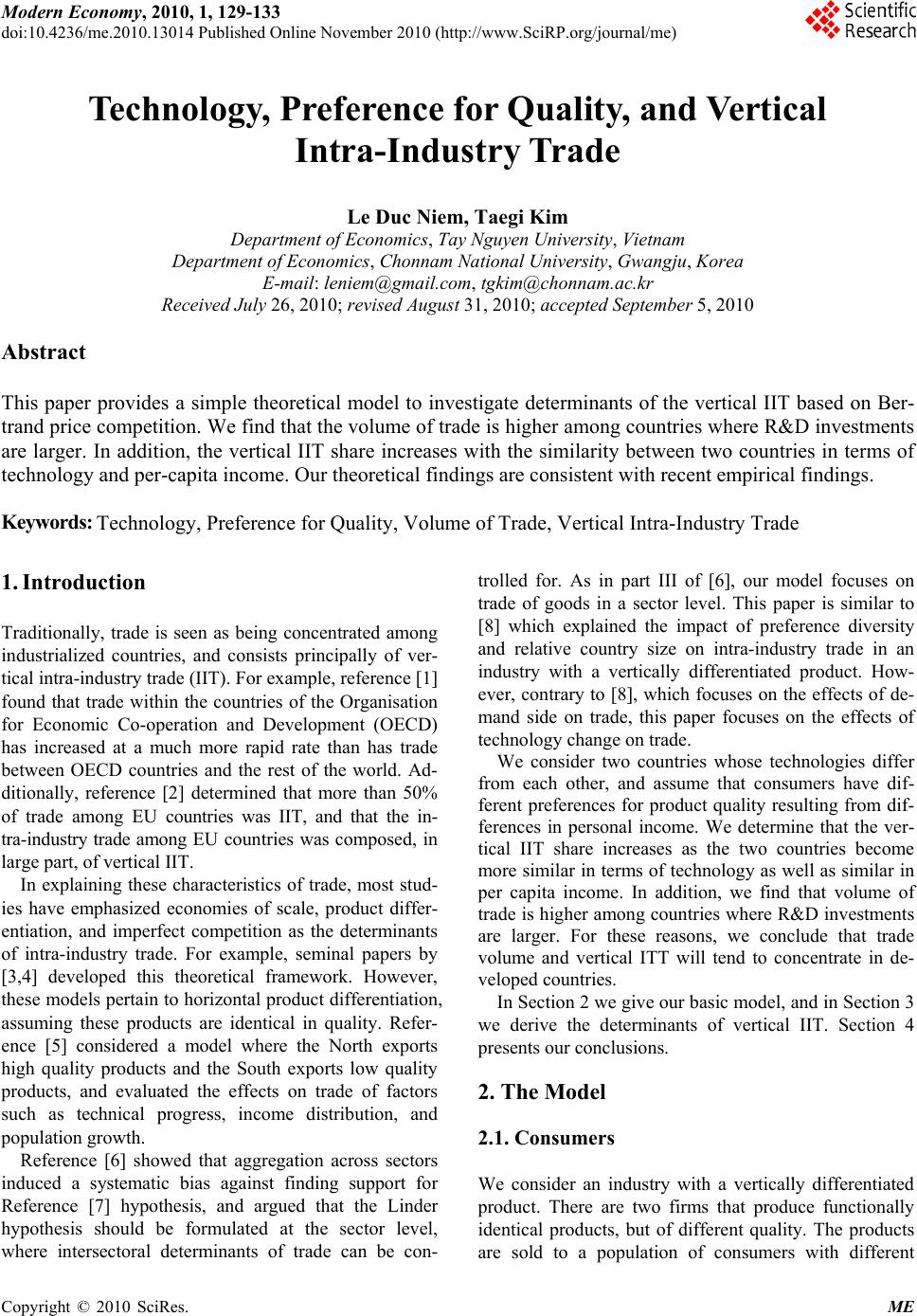Modern Economy, 2010, 1, 129-133
doi:10.4236/me.2010.13014 Published Online November 2010 (http://www.SciRP.org/journal/me)
Technology, Preference for Quality, and Vertical
Intra-Industry Tr ade
Le Duc Niem, Taegi Kim
Department of Economics, Tay Nguyen University, Vietnam
Department of Economics, Chonnam Nationa l University, Gwangju, Korea
Received July 26, 201 0; revised August 31, 2010; accepted September 5, 201 0
Abstract
This paper provides a simple theoretical model to investigate determinants of the vertical IIT based on Ber-
trand price competition. We find that the volume of trade is higher among countries where R&D investments
are larger. In addition, the vertical IIT share increases with the similarity between two countries in terms of
technology and per-capita income. Our theoretical findings are consistent with recent empirical findings.
Keywords: Technology, Preference for Quality, Volume of Trade, Vertical Intra-Industry Trade
1. Introduction
Traditionally, trade is seen as being concentrated among
industrialized countries, and consists principally of ver-
tical intra-industry trade (IIT). For example, reference [1]
found that trade within the countries of the Organisation
for Economic Co-operation and Development (OECD)
has increased at a much more rapid rate than has trade
between OECD countries and the rest of the world. Ad-
ditionally, reference [2] determined that more than 50%
of trade among EU countries was IIT, and that the in-
tra-industry trade among EU countries was composed, in
large part, of vertical IIT.
In explaining these characteristics of trade, most stud-
ies have emphasized economies of scale, product differ-
entiation, and imperfect competition as the determinants
of intra-industry trade. For example, seminal papers by
[3,4] developed this theoretical framework. However,
these models pertain to horizontal product differentiation,
assuming these products are identical in quality. Refer-
ence [5] considered a model where the North exports
high quality products and the South exports low quality
products, and evaluated the effects on trade of factors
such as technical progress, income distribution, and
population growth.
Reference [6] showed that aggregation across sectors
induced a systematic bias against finding support for
Reference [7] hypothesis, and argued that the Linder
hypothesis should be formulated at the sector level,
where intersectoral determinants of trade can be con-
trolled for. As in part III of [6], our model focuses on
trade of goods in a sector level. This paper is similar to
[8] which explained the impact of preference diversity
and relative country size on intra-industry trade in an
industry with a vertically differentiated product. How-
ever, contrary to [8], which focuses on the effects of de-
mand side on trade, this paper focuses on the effects of
technology change on trade.
We consider two countries whose technologies differ
from each other, and assume that consumers have dif-
ferent preferences for product quality resulting from dif-
ferences in personal income. We determine that the ver-
tical IIT share increases as the two countries become
more similar in terms of technology as well as similar in
per capita income. In addition, we find that volume of
trade is higher among countries where R&D investments
are larger. For these reasons, we conclude that trade
volume and vertical ITT will tend to concentrate in de-
veloped countries.
In Section 2 we give our basic model, and in Section 3
we derive the determinants of vertical IIT. Section 4
presents our concl usions.
2. The Model
2.1. Consumers
We consider an industry with a vertically differentiated
product. There are two firms that produce functionally
identical products, but of different quality. The products
are sold to a population of consumers with different

130 L. D. NIEM ET AL.
quality preferences. Each consumer may purchase a good
from one of the firms, or none at all.
The consumer’s utility when he consumes a good with
q units of quality and price p is described as follows:

ii
UJJq p (1)
This function is an indirect utility function of con-
sumer i, identified by the parameter i
J
. The population
of consumers is described by the parameter i
J
, and is
distributed uniformly between 0 and b. The parameter b
measures the heterogeneity in consumer preference for
quality. Consumers will decide to purch ase the good that
gives a higher and non-negative utility.
Subscripts H and L denote high and low quality prod-
ucts, respectively, and give the corresponding quality
level and price as
H
q,
L
q and
H
p,
L
p. We denote
L
H
J
to be the marginal consumer who is indifferent
with regard to consuming either of the two products.
That is, the consumer,
L
H
J
, satisfies
(, )(,)
H
HLL
. By Equation (1), the marginal
consumer
Uq pUqp
L
H
J
is defined as:


H
L
LH HL
pp
Jqq

 (2)
Some consumers do not wish to buy any goods at pre-
vailing prices. We denote
L
J
to be the consumer who is
indifferent in terms of purchasing a low quality product
and refraining from purchase. By Equation (1), this type
of marginal consumer is defined as:
L
L
L
p
Jq  (3)
All consumers having iLH
J
J will buy high quality
goods. All consumers having
L
HiL
J
JJ will buy
low-quality goods, and all consumers having iL
J
J

will not buy any goods1.
2.2. A Two-Country World
For the sake of simplicity, we assume a world of only
two countries: Home and Foreign. We assume that the
technology level of Foreign is higher than that of Home.
The quality level of the product will be determined by
the technology level. Therefore, the higher technology of
Foreign enables a firm to produce high quality products,
and the lower technology of Home enables a firm to
produce low quality products2. We assume that the qual-
ity of each product is a consequence of R&D investment,
but this quality cost has been sunk prior to price compe-
tition stage. In addition, production costs of these goods
are so small as to be negligible.
We let H
qQ

and L, where represents
the highest technology available in our world, and pa-
rameter k measures the technology similarity between
the two countries. Then k approaches 1, the two coun-
tries become more and more similar in terms of technol-
ogy. It is worthy noting that an increase in implies
that technology levels in bo th countries increase. Thus, Q
can be used as a proxy for our world technology level (or
regional technology level when we view the two coun-
tries as a region).
qkQQ
Q
The populations of consumers in Home and Foreign
are the same, and are normalized to 1. However, con-
sumers in each country differ in regard to their taste for
quality. Home consumers are distributed uniformly in the
interval of , and foreign consumers are distributed
uniformly in the interval of . We assume that
, which means that the range of preference for
quality is greater in Foreign than in Home. As conceptu-
alized by [9], a preference for quality is dependent on
consumers’ income; the more income a consumer has,
the more that consumer is willing to pay for any quality
level. For this reason, income level of Home (or Foreign)
can be considered a proxy for the (or ) variable.3
As preference diversity for quality is associated with
income, an assumption of implies that the in-
come level of Foreign is higher than that of Home. Thus,
we call the relative income level of the two
countries. It is noteworthy that and ap-
proaching 1 means the two countries become similar in
terms of income.
(0, )b
*
/hbb
*
(0, )b
b
*
bb
0
*
bb
*
b
1h h
Each country exchanges its products with the other
country.4 Home buys high quality products from Foreign,
and Foreign buys low quality products from Home.
Trade between the two countries can be illustrated as in
Figure 1.
2.3. Price Competition
Imagine a game as follows. There are no trade barriers
between Home and Foreign, and the two firms compete
simultaneously in price. We assume that no price dis-
crimination is possible because the goods can move
freely without any transportation costs between the two
countries.
3Consumer’s preference diversity is caused by differences in income.
Additionally, we assume that consumers in Home are uniformly dis-
tributed in [0,b] with regard to their preference. Thus, Home’s per
capita income is the average income of all of its consumers, which is
directly proportional to the average of consumer’s preference b/2 or
j
us
t
b.
4We consider an integrated economy as in [12] for our two country
world.
1See [10,11].
2This assumption is the same as [5], which assumes that the level o
f
p
roduct quality is determined by the level of technology.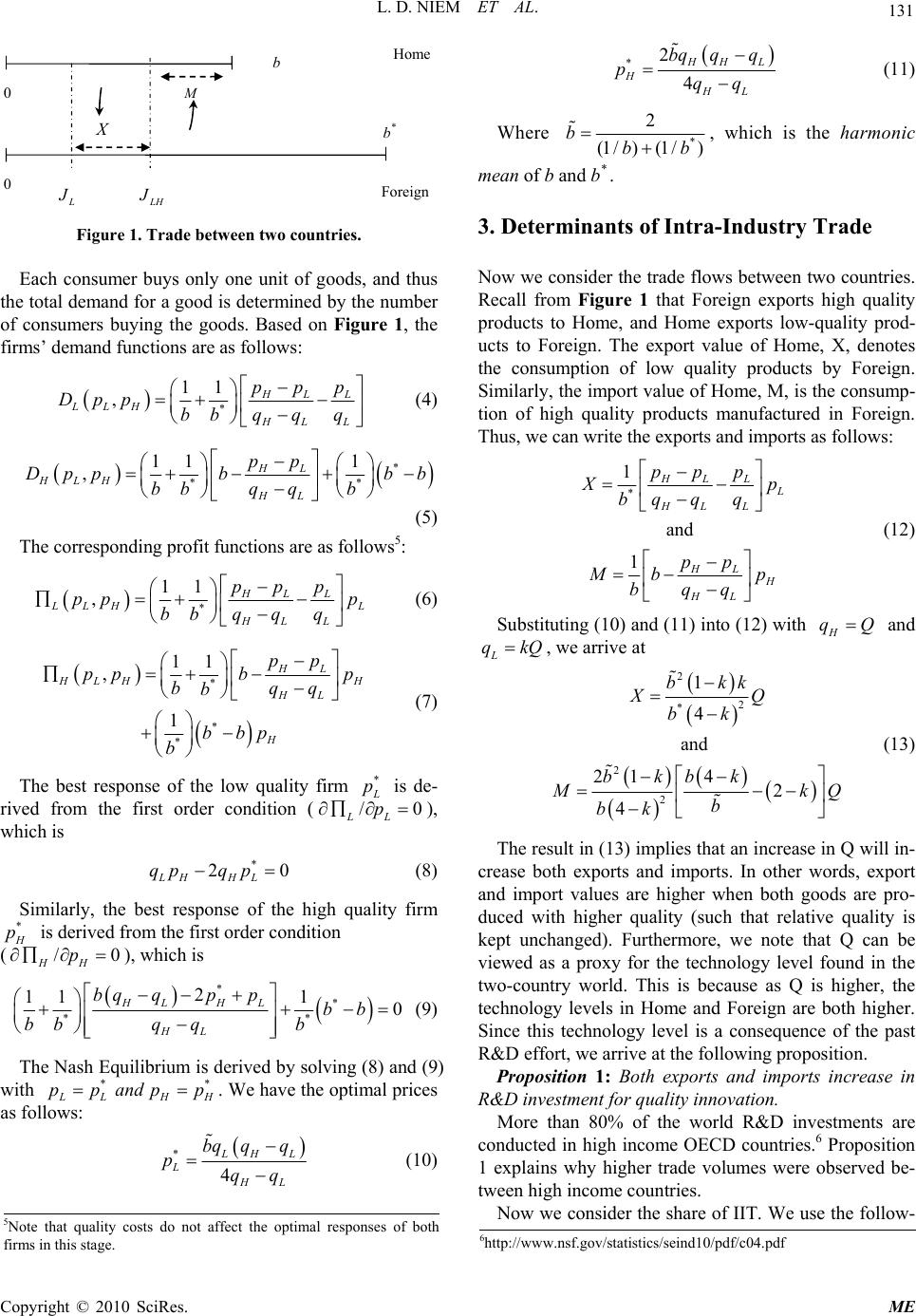

L. D. NIEM ET AL.
131
b
*
Home
Foreign
0
0
b
L
J
LH
J
M
X
Figure 1. Trade between two countries.
Each consumer buys only one unit of goods, and thus
the total demand for a good is determined by the number
of consumers buying the goods. Based on Figure 1, the
firms’ demand functions are as follows:

*
11
,HLL
LLHHL L
ppp
Dpp bqqq
b

 

 






 (4)


*
**
11 1
,HL
HLH HL
pp
Dpp bbb
bqq bb
 
 
 

 

 

(5)
The corresponding profit functions are as follows5:

*
11
,HLL
L
LH L
HL L
ppp
pp p
bqqq b
 

 






(6)


*
*
*
11
,
1
HL
H
LH H
HL
H
pp
ppb p
bqq b
bbp
b







 







(7)
The best response of the low quality firm *
L
p
LL
p is de- rived from the first order condition (),
which is /0 
*
2
LH HL
qpq p0 (8)
Similarly, the best response of the high quality firm
*
H
p

is derived from the first order condition
(), which is /
HH
p 0


**
*
2
111 0
HLH L
HL
bq qppbb
bqq
b

 



 



*
b

*
(9)
The Nash Equilibrium is derived by solving (8) and (9)
with *
L
LH
ppand ppH . We have the optimal prices
as follows:


*
4
L
HL
LHL
bq qq
pqq


 (10)

*2
4
H
HL
HHL
bq qq
pqq


 (11)
Where *
2
(1 /)(1 /)
bbb 
, which is the harmonic
mean of b and b* .
3. Determinants of Intra-Industry Trade
Now we consider the trade flows between two countries.
Recall from Figure 1 that Foreign exports high quality
products to Home, and Home exports low-quality prod-
ucts to Foreign. The export value of Home, X, denotes
the consumption of low quality products by Foreign.
Similarly, the import value of Home, M, is the consump-
tion of high quality products manufactured in Foreign.
Thus, we can write the exports and imports as follows:
*
1
and
1
HLL
L
HL L
HL
H
HL
ppp
X
p
qq q b
pp
M
bp
bqq

 












(12)
Substituting (10) and (11) into (12) with H qQ

and
L
qkQ

, we arrive at







2
2
*
2
2
1
4
and
214 2
4
bkk
XQ
bk
bkbk
M
kQ
b
bk














(13)
The result in (13) implies that an increase in Q will in-
crease both exports and imports. In other words, export
and import values are higher when both goods are pro-
duced with higher quality (such that relative quality is
kept unchanged). Furthermore, we note that Q can be
viewed as a proxy for the technology level found in the
two-country world. This is because as Q is higher, the
technology levels in Home and Foreign are both higher.
Since this technology level is a consequence of the past
R&D effort, we arrive at the following proposition.
Proposition 1: Both exports and imports increase in
R&D investment for quality innovation.
More than 80% of the world R&D investments are
conducted in high income OECD countries.6 Proposition
1 explains why higher trade volumes were observed be-
tween high income countries.
Now we consid er the share of II T. We use the follow-
5Note that quality costs do not affect the optimal responses of both
firms in this stage. 6http://www.nsf.gov/statistics/seind10/pdf/c04.pdf

L. D. NIEM ET AL.
132
ing Grubel-Lloyd index to compute the IIT index: countries are more similar with regard to per capita in-
come.

1
X
M
IIT
X
M

  (14) The propositions 2 and 3 above can be visually shown
in Figure 2, which is derived from equation (15). We
can observe that the IIT index increases with increasing
values of k, and that the IIT index becomes higher with
higher values of h. Remember that a higher value of k
implies more similar in terms of technology levels be-
tween the two countries, and that a higher value of h im-
plies more similar in terms of per capita income between
the two countries.
Substituting (13) into (14) and using *
b
hb , we get
2
4
kh
IIT hk 

(15)
Proposition 2: The IIT share is higher between coun-
tries with similar technology levels.
4. Conclusions
Proof: By formula (15), we have 0
IIT
k

. This
We have modeled the roles of R&D investments for
quality innovation and country similarities in per-capita
income and technology on vertical intra-industry trade.
Our principal findings are as follows.
means that the IIT index is large when k approaches 1
(recall that k is the relative similarity in tec hnology level
between the two countries, so k approaching 1 carries the
meaning that Home and Foreign are similar in terms of
technology). Put differently, IIT index is higher between
countries that have similar technology levels. Note that
whereas in proposition 1 trade volum e may be low,
proposition 2 implies the intensity of IIT (share) should
always be high when k approaches 1.
First, the volume of trade is higher among countries in
which R&D investments for quality innovation are
higher. Second, we found that the IIT index between
countries with similar levels of technology is high er than
that between those with differing levels of technology.
Finally, the IIT index was shown to be higher between
countries with similar levels of per-capita income.
Proposition 3: The IIT share is higher between coun-
tries with similar level of income. Countries with similar per-capita income or with
similar technology can be considered to be at similar
development levels. Thus, our theoretical findings may
help explain recent empirical findings that world trade is
more concentrated among the developed countries.
Proof: Formula (15) gives us 0
IIT
h

. This means
that IIT increases with increasing h. A higher h value
means that b and b* become more similar, or the two
Figure 2. IIT share and country similarity in technology and income.

L. D. NIEM ET AL.
133
5. Acknowledgement
We are grateful an anonymous referee for helpful com-
ments. We also wish to thank Kim Humphreys for Eng-
lish editing. All errors are ours.
6. References
[1] R. Bergoeing and T. J. Kehoe, “Trade Theory and Trade
Facts,” Federal Reserve Bank of Minneapolis Research
Department Staff Report No. 284, 2003.
[2] H. Gabrisch and M. L. Segnana, “Vertical and Horizontal
Patterns of Intra-Industry Trade between EU and Candi-
date Countries,” IWH-Sonderheft, Halle Institute for
Economic Research, 2003.
[3] P. Krugman, “Increasing Returns, Monopolistic Competi-
tion, and International Trade,” Journal of International
Economics, Vol. 9, No. 4, November 1979, pp. 469-479.
[4] K. Lancaster, “Intra-Industry Trade under Perfect Mo-
nopolistic Competition,” Journal of International Eco-
nomics, Vol. 10, No. 2, May 1980, pp. 151-175.
[5] H. Flam and E. Helpman, “Vertical Product Differentia-
tion and North-South Trade,” The American Economic
Review, Vol. 77, No. 5, December 1987, pp. 810-822.
[6] J. C. Hallak, “A Product-Quality View of the Linder Hy-
pothesis,” The Review of Economics and Statistics, Vol.
92, No. 3, August 2010, pp. 238-265.
[7] S. Linder, “An Essay on Trade and Transformation,”
Wiley, New York, 1961.
[8] T. Kim and L. D. Niem, “Product Quality, Preference
Diversity, and Intra-Industry Trade,” The Manchester
School, forthcoming, 2010.
[9] J. Gabszewicz, and J. F. Thisse, “Price Competition,
Quality and Income Disparities,” Journal of Economic
Theory, Vol. 20, No. 3, June 1979, pp. 340-359.
[10] X. Wauthy, “Quality Choice in Models of Vertical Dif-
ferentiation,” The Journal of Industrial Economics, Vol.
44, No. 3, September 1996, pp. 345-353.
[11] L. Beloqui and J. M. Usategui, “Vertical Differentiation
and Entry Deterrence: Reconsideration,” WP 2005-06,
Dept. Fundamentos del Analisis Economico II, Universi-
dad del Pais Vasco, 2005.
[12] E. Helpman and P. Krugman, “Market Structure and For-
eign Trade: Increasing Returns, Imperfect Competition
and the International Economy,” Wheatsheaf Books,
Brighton, 1985.