 Journal of Modern Physics, 2013, 4, 94-120 http://dx.doi.org/10.4236/jmp.2013.44A011 Published Online April 2013 (http://www.scirp.org/journal/jmp) Copyright © 2013 SciRes. JMP Grand Unified SU(8) Gauge Theory Based on Baryons which Are Yang-Mills Magnetic Monopoles Jay R. Yablon Schenectady, New York, USA Email: jyablon@nycap.rr.com Received January 15, 2013; revised April 22, 2013; accepted April 27, 2013 Copyright © 2013 Jay R. Yablon. This is an open access article distributed under the Creative Commons Attribution License, which permits unrestricted use, distribution, and reproduction in any medium, provided the original work is properly cited. ABSTRACT Based on the thesis that baryons including protons and neutrons are Yang-Mills magnetic monopoles which the author has previously developed and which has been confirmed by over half a dozen empirically-accurate predictions, we de- velop a GUT that is rooted in the SU(4) subgroups for the proton/electron and neutron/neutrino which were used as the basis for these predictions. The SU(8) GUT group so-developed leads following three stages of symmetry breaking to all known phenomenology including a neutrino that behaves differently from other fermions, lepto-quark separation, replication of fermions into exactly three generations, the Cabibbo mixing of those generations, weak interactions which are left-chiral, and all four of the gravitational, strong, weak, and electromagnetic interactions. The next steps based on this development will be to calculate the masses and energies associated with the vacuum terms of the Lagrangian, to see if additional empirical confirmations can be achieved, especially for the proton and neutron and the fermion masses. Keywords: GUT; SU(8); Yang-Mills; Baryons; Magnetic Monopoles; Nuclear Physics; Binding Energy; Protons; Neutrons; Fermions; Quarks; Electrons; Neutrinos; Leptons; Generations; Cabibbo Mixing; Chirality; Gravitation; QCD; Electroweak 1. Introduction In a recent paper [1], the author introduced the thesis that baryons, including protons and neutrons, are Yang-Mills magnetic monopoles. Based on this thesis, it was possi- ble to predict that the electron rest mass is related to the masses of the up and down quarks according to 3 2 2π edu mmm ((11.22) of [1]), with the factor of 3 2 2π emerging following a Gaussian integration over three space dimensions. Subsequent calculations showed that the best known values of the up and down masses in turn lead a binding energy of 7.667 MeV per the proton and 9.691 MeV per neutron yielding an aver- age binding energy of 8.679 MeV per nucleon ((12.6) through (12.8) of [1]), very much in accord with what is empirically observed, and to binding energies for 56Fe which were predicted to be extremely close to what is observed for that nuclide. Noting also that the deuteron binding energy is extremely close to what is known from best available data to be the mass of the up quark, we further hypothesized that these might be one and the same, which could be explained if the energies released during nuclear fusion are based on some form of “reso- nant cavity” analysis in which the discreet energies which are observed to be released are based on the masses of the quarks contained within the nucleons and nuclides. This led to a prediction that 56Fe has a latent available binding energy of 493.028394 MeV ((12.14) of [1]), which we then contrasted to the empirical binding energy of 492.253892 MeV. This small difference was understood as indicating that 99.8429093% of the avail- able binding energy predicted by this model of nucleons as Yang-Mills magnetic monopoles goes into binding together the 56Fe nucleus, and that the remaining 0.1570907% goes into confining the quarks within the nucleons. This in turn, lead us by the conclusion of [1] to a deepened understanding of how quark confinement is intimately related to nuclear binding and fission and fu- sion and the peak in per nucleon binding energies at 56Fe, and perhaps to an understanding of the so-called First ECM effect (see [1], pp. 62 and 66). A second paper [2] extended this analysis, and showed that based on this same “resonant cavity” analysis, the binding energies of the remaining 1s nuclides, namely 3H, 3He and 4He, can be predicted to at least parts per hun-  J. R. YABLON Copyright © 2013 SciRes. JMP 95 dred thousand and in most cases parts per million. This latter paper also showed that the observed neutron-pro- ton mass difference is predicted by the relationship 3 2 32 32π ud du MnM pmmmmm (in (7.2) of [2]) to better than 1 part per million. In Sec- tion 10 of [2], we explained why this should be regarded as an exact relationship, and therefore modified our ear- lier hypothesis that the deuteron binding energy is ex- actly equal to the up quark mass, into one in which these energies are very close—to just over 8 parts in ten mil- lion—but not exactly the same. In Section 9 of [2] we used these results to predict solar fusion energies solely from up and down quark masses, and found the results to also be in very tight accord with the observed data. The lesson taken from [1,2] together, is that empirical evidence strongly supports the thesis that Yang-Mills magnetic monopoles are in fact baryons on the basis of seven independent predictions which closely match the experimental data, specifically: 1) the electron mass in relation to the up and down masses, 2) the 56Fe binding energy specifically, and the per-nucleon binding energies on the order of 8.68 MeV in general, 3) the proton minus neutron mass difference, and 4-7) the four distinct nu- clide binding energies predicted for 4) 2H, 5) 3H, 6) 3He and 7) 4He. The study of solar fusion in Section 9 of [2] does not contain anything independent of the predictions 1) through 7), but rather applies several of these predict- tions in combination, and underscores that a “resonant cavity” analysis of nucleons and nuclides does consis- tently lead to empirically-accurate binding energies, evi- denced by all of predictions 3) through 7) above. While the theoretical foundation for all of these suc- cessful predictions was laid throughout [1], it was the field strength tensors for the proton and neutron, (11.3) and (11.4) of [1], reproduced below: P Tr 2, "" "" dduu dd uu F imm (1.1) N Tr 2, """ " uudd uu dd F imm (1.2) when used to calculate the energy according to 3 1Tr d 2 EFFx ((11.7) of [1]), which formed the specific basis for the calculations that led to all of these predictions. These field strength tensors, in turn, emerged as stable magnetic monopoles following specification of the SU(4)P “pro- tium” and SU(4)N “neutrium” gauge groups in Section 7 of [1], followed by breaking the symmetry of these groups using the baryon minus lepton number generator B − L via GUT vBL ((8.1) of [1]). So we take the thesis presented in Sections 7 and 8 of [1] that the protons and neutrons emerge following the B − L break- ing of the SU(4)P and SU(4)N groups to be supported by the compelling evidence of predictions 1) through 7), and so regard SU(4)P and SU(4)N as subgroups that do de- scribe the real physical universe, not just some arbitrary groups that may or may not appear in the natural world. In short, we take accurate empirical predictions 1) through 7) above as direct evidence of the physical real- ity of SU(4)P and SU(4)N. Based on all of the foregoing, we shall in this paper take SU(4)P and SU(4)N as physically-validated, reliable building blocks for developing a “Grand Unified Theory” (GUT) based on the empirically-confirmed thesis that baryons, including protons and neutrons, are Yang-Mills magnetic monopoles. 2. Unification and Grand Unification in Physical Science At least since the time when Isaac Newton hypothesized that the terrestrial “force” which caused an apple to fall from a tree was the same as the celestial “force” which guided the movements of the planets, unification has been a central objective of physical science. The pre- eminent scientist, entrepreneur and statesman Benjamin Franklin catapulted to fame when he realized that the terrestrial sparks he was creating in his laboratory were of a unified piece with the lightning from the heavens, and applied that understanding in a very practical way to develop lightning rods which cured an epidemic of mid- 18th century electrocutions throughout Europe brought about by the superstition of sending church bellringers to steeples at the highest place in town to clang large metal- lic bells to ward off the anger of the Gods every time a lightning storm approached. James Clerk Maxwell in 1873 elaborated what to that date was, and perhaps even to today’s date is, the preeminent physical unification and at least the very paradigm of unification, as he pulled together the disparate threads of Gauss, Faraday and Ampere into a unifying set of equations for electricity and magnetism. This was deepened a generation later with Einstein and Minkowski’s Lorentz-invariant unifi- cation of space and time. In these and similar endeavors the underlying theme has always been the same: to take what appear on their surface to be disparate natural phe- nomena, and acquire a deeper understanding which shows them to be governed by a single, common prince- ple. The success of past unifications leaves today’s gen-  J. R. YABLON Copyright © 2013 SciRes. JMP 96 eration of physicists with the firm conviction that further unifications can still be achieved, and that one day in the future, all of the laws of nature can and will be deduced from one common vantage point. After all, what is natu- ral science other than an endeavor to explain what is ob- served through our direct senses and the clever instru- mentation that extends our senses, by relating those ob- servations to mathematically precise laws of nature which apply consistently, uniformly and replicably, without exception, in the broadest possible range of cir- cumstances? So-called “Grand Unified Theories,” or GUTs, are part and parcel of this esteemed tradition, and are based spe- cifically on the advent of Yang-Mills gauge theories and the realization that these Yang-Mills theories have a re- markable capacity to explain what is observed in nature as evidenced though their already-successful application to weak and strong and electroweak interactions. The Georgi-Glashow SU(5) model [3] which was reviewed at some length in Section 8 of [1] was one of the first “GUTs” and is perhaps the best known. The basic idea of Georgi-Glashow and any other GUT is to be able to rep- resent all of the fermions which are observed in nature, and all of their interactions, using a single, simple gauge group with a symmetry which is then broken in one or more stages to arrive at the particle and interaction phe- nomenology observed in a laboratory setting. The fer- mions are the up and down quarks, the electron and neu- trino leptons, and ideally their higher-generational carbon copies distinguished from the first generation solely by larger mass. The generators of the gauge group represent “interactions” of which there are understood to be four: gravitational, strong, weak and electromagnetic. The ei- genvalues of the diagonalized generators of the gauge group, which are linearly related to discrete natural numbers such as 2 3 and 1 3 and 1 2 and −1 and 0, represent the “charges” of these fermions with respect to these interactions. A particular fermion may be associ- ated with a particular eigenstate (eigenvector) of a repre- sentation of the GUT gauge group if all of its eigenvalues for all of the generators match up with what are known to be the charges of that fermion with respect to all of these interactions. So, for example, an electron is by definition the fermion eigenstate for which the lepton number ei- genvalue L = 1, the baryon number eigenvalue B = 0, and the electric charge eigenvalue Q = −1. And the transi- tions/decays of a fermion from one eigenstate into an- other, or its interactions in a given eigenstate, lead to the mediating vector bosons of the theory. The trick in any GUT, is to characterize all of the interrelated charges of all of the fermions in the “simplest” way possible, to understand the stages and ways in which the symmetry of the group is broken starting at ultra-high energies and working down to energies which can be reached in a laboratory setting, and of course, to end up with some- thing that accurately comports with all observed empiri- cal data. With this in mind, and as used in the discussion here, we distinguish “GUTs” from “unified field theories” more generally, as that subset of unified field theories which is specifically centered on understanding fermions and their interactions via their discrete charges using Yang-Mills gauge groups, and on making whatever ob- servable predictions can be made based on such an un- derstanding. So, for example, Kaluza-Klein theory, which to this day represents an exceedingly elegant clas- sical unification of general relativity with Maxwell’s electrodynamics using a fifth spacetime dimension that from today’s vantage point is best understood as the “matter dimension” [4], is most certainly a form of “uni- fied field theory” (and one which in the view of this au- thor warrants more universal acceptance than it has at present, especially given that what we know of Yang- Mills gauge theory should permit both gravitation and electromagnetism in Kaluza-Klein form to be extended into non-Abelian domains). But Kaluza-Klein is not a GUT in the sense that GUTs are focused on the use of Yang-Mills gauge groups to represent fermions and their interactions, and Kaluza Klein, at least absent a Yang- Mills extension, has nothing to say about fermions. While one may define the term “GUT” more expansively to also include so-called “supersymmetric” theories, the foregoing defines by example, what we have in mind in this paper when referring to a “GUT”, as opposed to a “unified field theory” without the GUT qualifier. The Galilean foundation for all of modern science is that theory must be the confirmed by observation, and that the goal or at least an important by-product of theory is to systematically explain observation. For physical theorists, the pursuit is about systematically compre- hending nature and confirming that comprehension based on experimental data, or as Hawking and Einstein have more loftily put it, “reading the mind of God.” Because GUTs necessarily theorize about the behavior of nature at ultra-high energies such as 1015 GeV and even higher that are unlikely to ever be reached by human experi- mentation under any foreseeable circumstances (with the possible exception of what we can learn by peering back billions of years through astronomical telescopes), such GUT theories necessarily opine on physics that may for- ever be beyond the reach of direct experimental confir- mation. So the only way to discern the primacy of one GUT over another is indirectly, by virtue of what it pre- dicts about low energy phenomenology that we can or may soon be able to observe. So as we consider how to construct the “puzzle” which is a GUT and decide what “pieces” to use in that puzzle, we want to start with puz-  J. R. YABLON Copyright © 2013 SciRes. JMP 97 zle pieces that already are solidly-grounded in empirical observation. Based on the seven independent predictions enumer- ated in the last section which closely match the empirical nuclear binding and related data based on the thesis that baryons are Yang-Mills magnetic monopoles, the GUT that we develop here will start with the SU(4)P and SU(4)N gauge groups developed in Sections 7 and 8 of [1], knowing that these groups now have been validated by over half a dozen independent pieces of empirical data from nuclear and particle physics. Additionally, because we have shown in [1,2] how to connect these gauge groups to energy numbers which can be and indeed have been empirically confirmed, an important objective in developing a GUT on the basis of SU(4)P and SU(4)N is to lay the foundation for perhaps obtaining additional, similar, successful predictions of other known energies which have been crying out for theoretical understanding for decades, most particularly, and most importantly, the free proton and neutron masses, and the observed fer- mion masses. If it should be possible on the basis of a particular GUT to make accurate predictions of the proton and neu- tron and/or fermion masses, then even absent the ability to ever directly observe the 1015 GeV and higher energy phenomena which lead to these predictions, such predict- tions would certainly be solid evidence, albeit through indirect inference rather than direct observation, that such a GUT has also explained to us how nature behaves behind the veil of energies that we shall most certainly never get to directly observe (again, with possible astro- nomical caveat). In other words, because a GUT, by its very nature, seeks to reach into energy domains that will likely be forever beyond human reach, it must fulfill the Galilean project by accurately explaining all of the masses and energies that we do observe through the instrumentation that does rest within our grasp, while at the same time teaching us about physics at energies that we shall likely never have the capacity to see directly. It is the prediction of the energies and masses we do observe, that gives us some measure of confidence that we are not being led astray by what the GUT tells us about the physics of un- reachable energies. To use a different metaphor, GUTs seek to teach us about an entire iceberg, most of which we shall never be able to observe. So what the GUT teaches us about the tip of that iceberg which we can see, must be solidly-confirmed by empirical data every step of the way for us to have some confidence in what it teaches us about the rest of the iceberg which will forever remain out of sight. Based on the foregoing, the purpose of this paper is to develop a GUT rooted in the thesis that baryons are Yang-Mills magnetic monopoles and the seven success- ful predictions which have already emanated from that thesis in [1,2], and to lay the foundation for additional mass and energy predictions, including those of the free proton and neutron and the fermion masses. 3. Some Clues for Pursuing the Proton, Neutron and Fermion Masses Before we can make predictions of the proton and neu- tron and fermion masses, we must construct a reliable, empirically-grounded GUT, and we must know how to break its symmetry. Why do we say this? We have already shown in [2] how the nuclear binding energies in the 1s shell arise from using the field strength tensors (1.1) and (1.2) to calculate an energy 3 gaugedEx L via the pure gauge terms in the La- grangian (3.8) of [2]: 3 2 binding 12π 2ABBAAA BB FF FF L, (3.1) together with components , ud mm and ud mm of the outer product ABCD E ((4.9) through (4.11) of [2]). But these binding energies are calculated using only the pure gauge field terms (3.1) of the Lagrangian developed in (3.12) of [2], written with the terms slightly regrouped: 3 2 3 2 322 2 322 2 12π 2 2π 2π 11 2π. 22 ABBAAA BB AB AA ABB AB BAAA BB AB BAAA BB FF FF DD DD L (3.2) We have not yet even begun to develop these other terms at all, yet it is made very clear by the development in [1,2] that additional energy numbers can and will arise from complete development of these terms. So, we must develop these additional terms and we will look to them to perhaps lead us to the proton and neutron and fermion masses. But because all of these terms contain the vac- uum , the actual numeric energy values we obtain from these -containing terms will depend upon the GUT gauge group we choose, and upon its vacua and how these vacua are used to break symmetry. (We use the plural vacua because we have in mind breaking symmetry in sequence using the Planck vacuum on the order of 1019 GeV, so called GUT vacuum on the order of 1015 GeV, and the Fermi vacuum vF = 246.219651 GeV used to break electroweak interactions to electro- magnetic interactions via 21 1 WY EM SU UU .) For example, given from (3.11) of [2] that:  J. R. YABLON Copyright © 2013 SciRes. JMP 98 , EF EF F DiG , (3.3) we see that terms in (3.2) with DD will mix gauge fields G with vacuum fields . So whereas the pure gauge terms (3.1) led to expressions such as (4.9) and (4.10) of [2], namely: 33 3 22 1 2π2πd 2 00 00 0000, 00 00 PABCDPAB PCD dd uu uu EFFx mm mm mm (3.4) 33 3 22 1 2π2πd 2 00 00 0000, 0000 NABCDNAB NCD uu dd dd EFFx mm mm mm (3.5) we should be alert to opportunities to develop mixed gauge field/vacuum terms where one of these matrices is replaced by a vev, especially the Fermi vev vF = 246.219651 GeV, so we can develop an energy “tool- box” with such expressions as u vm and d vm . Why the Fermi vev? And why these square root expres- sions? Because numerical inspection of the square roots of the three main masses in (4.11) of [2] used to calculate binding energies throughout [2], times the square root of the Fermi vev, shows that: 739.960397 MeV u vm , (3.6) 1099.12211 MeV d vm , (3.7) 901.835259 MeV ud vmm . (3.8) These clearly are at exactly the right order of magni- tude to explain the free proton and neutron masses M(p) = 938.272046(21) MeV and M(n) = 939.565379(21) MeV, if and when we can put (3.6) through (3.8) and like expressions into the right context and obtain the right coefficients. And where do such coefficients come from? The generators of a GUT! (The author’s subsequent pa- per in this same special issue of JMP starts with (3.8) to indeed successfully explain the free neutron and proton rest masses.) So the proton and neutron masses, via the order of magnitude analysis above, straddle right down the mid- dle of the Fermi vev and the masses of the quarks. One should therefore be on the lookout for ways to exploit this via the “mixed” gauge field vacuumG terms in Lagrangian (3.2). And as noted at the end of Section 10 of [2], one should keep in mind that relation 3 2 32 32π ud du MnM pmmmmm for the free neutron-proton mass difference now allows us to find the neutron and proton masses individually, so long as we can find sum expression which involves the sum of these masses. So it may well be that our target should be nMp or some multiple thereof (perhaps the 4He alpha nucleus studied extensively in [2]?) rather than either of these masses individually. For another example, we go all the way back to (2.1) of [1], Maxwell’s charge equation: 2 , , JF DG GiGG J mGG iGG (3.9) with DiG , and where in the final term we have hand-added a “Proca mass.” Based on (3.3), we can readily specify an analogous field equation: 2 , , JF DiG JmiG (3.10) for a Yang-Mills (non-commuting) scalar field with a scalar source J. In fact, this is just the Klein-Gordon equation for a non-Abelian (non-commuting) Yang-Mills scalar field with a non-zero scalar source, into which we have hand-added a Proca mass in the usual way. The rea- son this is of interest is that a central step in Section 2 of [1] was to develop the inverse GIJ and then intro- duce fermion field wavefunctions via J , so that we went from GIJ I . But we can follow an analogous path with (3.10) by building scalar source J out of fermions via J . Then we can develop an inverse via J and follow the analogous progression IIJ . Consequently, the terms of the Lagrangian (3.2) quadratic in the scalar field can be developed as 22 2 IIJ , and then we can follow the path of section 3 of [1] by em- ploying spin sums 2 uu Nmm , with the full progression 22 2 22 II I J Nm m Then, if we pursue the same course of development as in [1] from start to finish, when we finally reach the counterpart of (11.19) of [1] and collapse the propagators so that interactions occur essentially at a point, we will end up with a Lagrangian term of the schematic form: 22 22 II I f J Nm mm L (3.11) But this is the form of a Fermion mass term in a La-  J. R. YABLON Copyright © 2013 SciRes. JMP 99 grangian, with the mass of the fermion specifically iden- tified with 22 I f mNmm. Concurrently, the vev v should also enter into this when we break symmetry with a generator G by setting vG . So this is a pos- sible prescription, using the terms in (3.2), for revealing a fermion rest mass out a Lagrangian while preserving gauge symmetry and thus maintaining renor- malizability! But because the specifics of all of this center around the vacua , it becomes essential to have the right GUT gauge group, and to know how to break its symmetry in appropriate sequence. As noted above, to do this, we begin to develop a GUT gauge group using the SU(4)P and SU(4)N gauge groups developed in Sections 7 and 8 of [1], knowing that these groups now have been vali- dated by over half a dozen independent pieces of empiri- cal evidence from nuclear and particle physics. We build upon these empirically-validated puzzle pieces in the hope that this run of positive empirical predictions will continue with the masses and energies predicted by the terms in (3.2) which include the vacua . 4. An Unbroken SU(8) GUT Group which Accommodates All Fermions and Left and Right-Chiral States, All Interactions, Three Generations, and an Idiosyncratic Neutrino, with Nothing Missing and Nothing Superfluous The proton and the neutron, of course, form an SU(2) weak isospin doublet ,pn with 311 , 22 I , re- spectively. But both the proton and the neutron are com- posite entities comprising three quarks, and as we have argued and indeed supported with empirical nuclear binding data, they are Yang-Mills magnetic monopoles. So really, the proton/neutron doublet is a doublet of trip- lets, ,,, ,,duuudd . And the left-chiral weak iso- spin quantum numbers 3 associated with this triplet doublet are 111111 ,,,, 2222 2 2 . In Section 7 of [1], we demonstrated that at ultra-high GUT energies the proton was part of a larger gauge group which we dubbed the SU(4)P “protium” group which includes the proton and the electron, and that the neutron was similarly part of a larger gauge group we dubbed the SU(4)N “neutrium” group which includes the neutron and the neutrino. As we then showed in Section 8 and specifically (8.1) of [1], these two groups are broken by a vacuum GUT vBL of a “baryon minus lep- ton number” generator 15 8 3 BL such that a pro- ton triplet ,, GB duu is separated from the electron for SU(4)P and a neutron triplet ,, GB udd is separated from the neutron for SU(4)N, and each triplet becomes part of a topologically-stable magnetic monopole. It was on the basis of these proton and neutron triplets broken out from SU(4), that we successfully rendered the seven predictions summarized in Section 1, and also correctly derived the fusion energy released during the solar fis- sion cycle strictly as a function of the up, down and elec- tron fermion masses. So these triplets and the SU(4)P and SU(4)N groups in which they are embedded would appear to be very solid puzzle pieces for constructing a larger GUT which is well-grounded empirically. That is exactly what we shall do here. Normally, one works from the phenomenological gauge group 321 CWY SU SUU and tries to find larger simple groups G which embed all of these and their associated fermions. The SU(5) model of Georgi- Glashow [3] reviewed at some length in Section 8 of [1] is a paradigmatic example. Here, we shall start with SU(4)P and SU(4)N which we know lead to accurate binding energy predictions, and seek to construct a larger simple gauge group which includes these two groups, and which also encompasses the usual phenomenological gauge group 321 CWY SU SUU . The group we shall choose? 84 4 P SU SUSU. This is a larger group than SU(5), but as we shall see, it brings with it numerous benefits including 1) the ability to ac- commodate a non-zero neutrino mass and thus right- handed chiral neutrinos which are omitted from SU(5); 2) the ability to accommodate all flavors and colors of fer- mion, as well as protons and neutrons, all in the funda- mental group representation (SU(5) splits the fermions into a fundamental 5 and a non-fundamental 10 repre- sentation while omitting the right-chiral neutrino); 3) the ability to accommodate different left and right-handed chiral projections with respect to weak hypercharge Y and weak isospin I3, for all fermions; 4) a solution, at long last, to the mystery of fermion replication into ex- actly three generations, and 5) interaction generators that may well be associated with gravitation based on the manner in which the elusive neutrino stands alone with respect to all other fermions by having an exceedingly tiny neutrino mass that is orders of magnitude smaller than the masses of the other fermions, and based on the ability to finally understand the origins of fermion gen- eration replication. We construct this SU(8) group by establishing a fun- damental representation containing the fermion octuplet ,,, ,,,, RGB RGB udd eduu . The neutron triplet ,, GB udd and proton triplet ,, GB duu are design- nated in separate parenthesis for visual emphasis, and as we can see, the neutrium group ,,, GB ud d occupies the first four members of this octuplet and the protium group ,,, GB eduu occupies the last four members. Of course, what really counts are the quantum numbers,  J. R. YABLON Copyright © 2013 SciRes. JMP 100 so let’s now turn to those. In (7.1) of [1], we established that for the protium quadruplet, the electric charge generator could be speci- fied by 8158 22 2 33 QBL . But in (7.3) of [1], we were required to use a different electric charge generator, namely 8 2 3 Q for the neutrium quadruplet. This if OK when the proton and electron are treated separately from the neutron and neutrino, and this was good enough to get us over half a dozen good bind- ing energy predictions and other empirically-supported relationships. But once we put all these fermions to- gether into one octuplet representation of a unifying group this is no longer OK, and we need to define a new electric charge generator that works uniformly for all of the fermions in the group. So let us now see exactly how we can put these two groups together and what this implies for the nature of the GUT that does so. SU(8) of course contains seven diagonalized 8 × 8 generator matrices, so rather than take up visual space with seven 88 matrices in which all but the diagonal elements are zero, let us construct this group using the tables below which convey the same information more compactly in an easier-to-follow form. First, as just noted, the electric charge generator is 8158 22 2 33 QBL for SU(4)P, while it is 8 2 3 Q for SU(4)N. So if we lay out the eight fermions of this octuplet in a vertical column and show the three generators 15 8 3 ,, of SU(4) in the first three columns (we actually show 15 8 3 BL which is merely a linear multiple of 15 ), and then show generators for electric charge Q, right-chiral weak hypercharge 2 R YQ, left chiral weak hypercharge L YBL , and right-chiral weak isospin 30 R I , which are all linear combinations of one or more of the three generators 158 3 ,, , we end up with Ta- ble 1 below. In Table 1 below, we have segregated the SU(4)P and SU(4)N generators 158 3 3,, 8BL from the remaining generators, so that we can clearly see that there are three linearly-independent degrees of freedom. The remaining generators for Q, YR, YL, are all linear combinations of the first three generators, and so provide no additional degrees of freedom, while 30 R I can be trivially obtained from any other generator using the co- efficient 0. We shall wish, in the course of our analysis, to maintain a focus on the independent degrees of free- dom. What makes the upper neutrium quadruplet not unified with the lower protium quadruplet is the fact, as mentioned above, that although all the other generators have the same form (i.e., are invariant) as between the Table 1. Fermions and generators of SU(4)N and SU(4)P. Linearly Independent Degrees of Freedom Linear Combinations 15 8 3 BL 8 3 8 2 3 Q 2 R YQ L YBL 3 ν 1 0 0 0 0 1 0 uR 1 3 1 3 0 2 3 4 3 1 3 0 dG 1 3 1 23 1 2 1 3 2 3 1 3 0 dB 1 3 1 23 1 2 1 3 2 3 1 3 0 " " " 8 2 3 QBL " " " e 1 0 0 1 2 1 0 dR 1 3 1 3 0 1 3 2 3 1 3 0 uG 1 3 1 23 1 2 2 3 4 3 1 3 0 uB 1 3 1 23 1 2 2 3 4 3 1 3 0  J. R. YABLON Copyright © 2013 SciRes. JMP 101 upper and lower quadruplets as denoted by the “dittos”, the electric charge generators are defined by different linear combinations. So electric charge Q is not an in- variant as between these two quadruplets. It is worth not- ing that for all of these fermions, L YBL, so Y is not itself a linearly-independent generator from 15 . The one generator that we do not see explicitly repre- sented in the above, of course, is the generator 31 2 L I of left-chiral weak interaction, and this is related very intimately to the different Q generators as highlighted above. So, let us now a) introduce 3 and b) use this 3 in combination with YL which happens to be equal in all cases to BL, to specify 3 2 L QY I as is ordi- narily done in electroweak theory. Then, having Q in hand, and given 30 R I, we may further specify 2 R YQ if we insist on the chiral-invariant relationship 33 22 LR R QYI YI . So we now take Table 1 above, introduce all seven of the SU(8) diagonalized generators with the normalization 21 Tr 2 i , and specify suitable linear combinations of these. Then, we review not only how this accommodates the fermions and generators in Table 1 above, but also the new interaction generators that are introduced and their possible physical significance. Aesthetically, is very simple and natural for the eight fundamental flavors and colors of fermion ,,,,,,, GB RGB uddeduu to each be made a member of the fundamental representation of SU(8). And, be- cause one does have eight fermions in nature (per gen- eration), a natural question is, why not use SU(8)? Some- times, what appears to be the simplest approach really is the simplest approach, and leads to the best results, and we don’t have to try to unnaturally “squish” eight fer- mions into a smaller group like SU(5) and then lose the right-chiral neutrino and split the representations. In this regard, the question we shall explore largely throughout the rest of this paper—which is one of the reasons why one might not use SU(8)—is whether SU(8) is simply too large and can or ought to be made smaller. (We shall answer this question, “no”!) By “too large,” we refer not to aesthetics, but to superfluity: does this group introduce any extra, superfluous particles or interactions which simply do not appear anywhere in the natural world. Put concisely, the underlying question is this: is SU(8) sufficient, and is everything in SU(8) necessary? Does it yield everything, and not one iota more? (We shall answer these questions, “yes”!) Specifically, in going from two disjoint SU(4) groups in Table 1 to one unified SU(8) group in Table 2, we have gone from three independent generators 15 8 3 ,, to seven. Out of these four new generators, we have left three of these, 6348 35 ,, , in their “native” form with- out alteration, pending further exploration of these gen- erators below. The fourth new generator, 24 , we do not show explicitly. Rather, we use the degree of freedom provided by 24 to introduce the left-chiral weak isospin generator 3 , which we define as a linear combination of six of the seven “native” generators according to: Table 2. Fermions and generators of SU(8). Linearly Independent Degrees of Freedom Linear Combinations 63 48 35 3 L 8 3 Y Q Y 3 ν 17 228 0 0 1 2 1 0 0 1 0 0 0 uR 1 228 16 221 0 1 2 1 3 1 3 0 1 3 2 3 4 3 0 dG 1 228 1 221 15 215 1 2 1 3 1 23 1 2 1 3 1 3 2 3 0 dB 1 228 1 221 1 215 1 2 1 3 1 23 1 2 1 3 1 3 2 3 0 e 1 228 1 221 1 215 1 2 1 0 0 1 1 2 0 dR 1 228 1 221 1 215 1 2 1 3 1 3 0 1 3 1 3 2 3 0 uG 1 228 1 221 1 215 1 2 1 3 1 23 1 2 1 3 2 3 4 3 0 uB 1 228 1 221 1 215 1 2 1 3 1 23 1 2 1 3 2 3 4 3 0  J. R. YABLON Copyright © 2013 SciRes. JMP 102 36348 35 24 158 24 2 72115 222 . 53 3 L I (4.1) One can readily check that 311111111 diag,,,,,,, 22222222 L I as in Table 2. Now, for the bottom quadruplet with ,,, GB ed u u, we have 15 2 23 BL as before. But this relation- ship needs to be replicated out of the native generators for the top quadruplet ,,, GB udd as well. This is realized by the following linear combination of native generators: 6348 35 24 15 4443 95 7321 22 2 2 35 3 BL (4.2) So we use (4.1) and (4.2) above to account for the two linearly-independent degrees of freedom in 24 and 15 . It is easy to check as in Table 2, that 111 111 diag 1,,,,1,,, 333 333 BL . Similarly, we cannot use 8 alone, but must dupli- cate this as well for the top quadruplet ,,, GB ud d . This is achieved by defining a 8 generator: 848 35248 72 2 315 35 . (4.3) As required from Table 2, a check finds that 8 diag 11 111 1 0,, , ,0,, , 3232332323 Finally, and similarly, we need to define a 3 ac- cording to: 335243 32 55 . (4.4) This yields 31111 diag0, 0,,, 0, 0,, 2222 as in Table 2. The foregoing, (4.1) through (4.4), account for four of the seven linearly-independent degrees of freedom in SU(8). We have yet to explore the three na- tive-form generators 63 48 35 ,, . From here, we define several other generators which are linear combinations of (4.1) through (4.4). First, via (4.2), we define: 63 48 3524 15 44 7321 43 228 95 353 L YBL (4.5) which happens to be exactly equal to BL in (4.2) and so is not linearly independent. But Y is non-chiral, i.e., it only applies to left-chiral projections. Next, we use (4.5) and (4.1) to define the electric charge generator in the usual manner, via: 333 483524 15 8 11 22 27 422 33 35 315 22 233 LL LR QYIBLII (4.6) One can check to see that 211 122 diag0,, , ,1, ,, 333 333 Q , as required by Table 2. In the third expression we make use of 30 R I , to show by way of contrast that Volo- vok’s Equation (12.8) in [5] also leads via a different route to the exact same 33 1 2 R QBLII . Next, we formally specify that the right-chiral genera- tor 30 R I (4.7) is to be zero for all the fermions so that only left-chiral particles will interact weakly. At the same time we insist that the electric charge generator 33 11 22 LRR QYIYI (4.8) is to be defined as chiral symmetric for all fermions. This chiral insistence together with (4.6) and (4.7) finally leads to: 4835 24 15 8 47 842 233 35 315 24 433 R YQ (4.9) So at this point, all of the known quantum numbers of the fermions are fully specified, including the left and right chiral projections for Y and I3. The fermions all re- side in the fundamental representation of SU(8), and the proton and neutron are represented as well in the way  J. R. YABLON Copyright © 2013 SciRes. JMP 103 that we have ordered the fundamental representation. And, while all of the foregoing certainly accounts for the observed fermions and their quantum numbers, we still have three extra linearly-independent degrees of freedom, which we can and do choose to associate with the gen- erators 6348 35 ,, we have left in their native state. Now we return to the critical question: With these three apparently superfluous degrees of freedom, does SU(8) provide too much freedom? Does SU(8) provide more than what is necessary? Might we find some way, in the spirit of Georgi Glashow SU(5), to “squish” these fermions into a smaller group and take away some of this apparently-superfluous freedom? The answer is, no! And the reason is that this extra freedom is not superfluous, but is actually fully accounted for in the known particle phenomenology, and particularly, in the odd quirks of the neutrino and in the replication of fermion generations. Let us see how. First, the neutrino. One of the very perplexing features of the neutrino is that it has almost no mass, and is mad- deningly-elusive. While the electron and the quarks do have different masses from one another, the neutrinos are in a league of their own, by orders of magnitude. The neutrino mass is almost zero, which means that it travels at very close to the speed of light. Because of the equivalence of gravitational and inertial mass, the fact that the mass of the neutrino is so very different from that of all the other fermions means that in some rough man- ner of speaking, it is gravitating differently as well. For example, the mass of the electron’s neutrino is less than 2 eV [6], while the electron itself has a mass of about 511 KeV, which is over 250,000 times as large. This is of a totally different nature, involving completely different orders of magnitude, than 4 351853369 ue mm . and 9 601723351 de mm . which are the relationships be- tween the quark masses and the electron masses based on the quark masses arrived at in (10.3) and (10.4) of [2]. This appears to make the neutrino qualitatively different from all the other fermions, and we need to pinpoint the origins of this difference. Now consider the 63 in Table 2 and the fact that 63 1 47 for all of the up and down quarks and the electron, but that 63 7 47 has a completely differ- ent value for the neutrino. Moreover, not only is the magnitude different by 7 to 1, but even more importantly, the sign is different. Indeed, that is why we chose to place the neutrino as the very top member of the SU(8) fermion octuplet. That means that the neutrino will in- teract completely differently under the interaction asso- ciated with 63 —whatever that interaction may be— from any other fermion. But if there is any interaction under which the neutrino behaves differently than all the other fermions, it is the gravitational interaction, because the most pronounced way in which the neutrino differs from the other fermions is via its ghostly mass and thus its ghostly way of gravitating. Further, we know on gen- eral principles that for any Yang-Mills gauge group which unifies gravitation with the other three interactions, there will have to be at least one degree of freedom given to the gravitational interaction. The only question is where and how this appears. So, we now make a preliminary association of the 63 generator with a degree of freedom for a gravita- tional interaction, and we do so in a way that bakes in for the neutrino, an entirely different way of gravitating and thus displaying its mass, than any other fermion. So, now we have accounted at least in a general way (which we shall seek to deepen in the upcoming discus- sion) for all four of the known interactions, but we still have two more degrees of freedom unaccounted for, namely, those provided by 48 35 , . What are we to make of these? This brings us again to the question: does this not give us too much freedom? And again, the an- swer is, no! We still have to account for the replication of fermions into three generations, which is another oddity of the material world almost as mysterious as the oddities of the neutrino just discussed. Let’s ask the question directly: even if 63 is related to gravitation and can explain why the neutrino behaves so differently from all the other fermions, 4835 , still give us two apparently super- fluous degrees of freedom. What does this mean? What can we do with those extra two degrees of freedom? And specifically, might they be origin of generation replica- tion? Any time we have two degrees of freedom such as are provided by 48 35 , , it is possible to construct three eigenstates out of those degrees of freedom. So, let us do just that, and label these states ,,e as in Figure 1 below. We use “primes” in these generators, because if they do represent degrees of freedom associated with genera- tion replication, they do not act in same way as the re- maining generators 6324 15 83 ,,,, in Table 2. These other five generators represent a “vertical” sym- metry wherein each of the eight fermions is distin- guished from one another by different quantum numbers. But the appearance of three generations in which the quantum numbers are identical from one generation to the next, and in which for a given fermion, generation is distinguished exclusively by rest mass, is a horizontal symmetry. And it is for and to this horizontal symmetry, that we shall develop and devote the generators 48 35 , . Now, in the forthcoming discussion, we shall seek to uncover in detail, the particular mechanism by which  J. R. YABLON Copyright © 2013 SciRes. JMP 104 these two generators 4835 , separate themselves from the remaining vertical generators 63 383 ,,, ,IBL to situate themselves horizontally. The only point being made at the moment, is that two extra generators in Yang-Mills theory, such as 48 35 , , provide enough freedom to support three distinct states as in Figure 1. And these three states will come equipped with their own 3 × 3 unitary matrices U to mix these states. And, if we are asking ourselves whether the extra two generators 48 35 , provide too much freedom at the same time that we are seeking an explanation of the three fermion gen- erations, and given that those two extra generators pro- vide precisely the freedom needed to allow each particle to exist in one of three additional horizontal generational states, then perhaps these are not superfluous after all, but are instead the source of the generations. In that case, SU(8) becomes a perfect fit, large enough to accommo- date all that is observed including the idiosyncratic be- havior of the neutrino and the replication of fermion generations, and not one bit larger so as to contain any- thing superfluous that is not observed. So in Table 3 below, we shall use the schematic sym- bol to denote a visual shorthand for Figure 1 below: a condensed symbol that represents two degrees of free- dom which are used to provide three distinct states ,,e which appear in Figure 1. And, let us replace the generators 4835 , with this schematic to represent the horizontal symmetry of generation replication. Thus, we now rewrite Table 2 in the form of Table 3 as shown below. Figure 1. Three generation eigenstates constructed from 48 and 35 . Table 3. Fermions and generators of SU(8), with generation replication. Linearly Independent Degrees of Freedom Linear Combinations 63 48 35 , 3 L 8 3 Y Q Y 3 ν 17 228 1 2 1 0 0 1 0 0 0 uR 1 228 1 2 1 3 1 3 0 1 3 2 3 4 3 0 dG 1 228 1 2 1 3 1 23 1 2 1 3 1 3 2 3 0 dB 1 228 1 2 1 3 1 23 1 2 1 3 1 3 2 3 0 e 1 228 1 2 1 0 0 1 1 2 0 dR 1 228 1 2 1 3 1 3 0 1 3 1 3 2 3 0 uG 1 228 1 2 1 3 1 23 1 2 1 3 2 3 4 3 0 uB 1 228 1 2 1 3 1 23 1 2 1 3 2 3 4 3 0 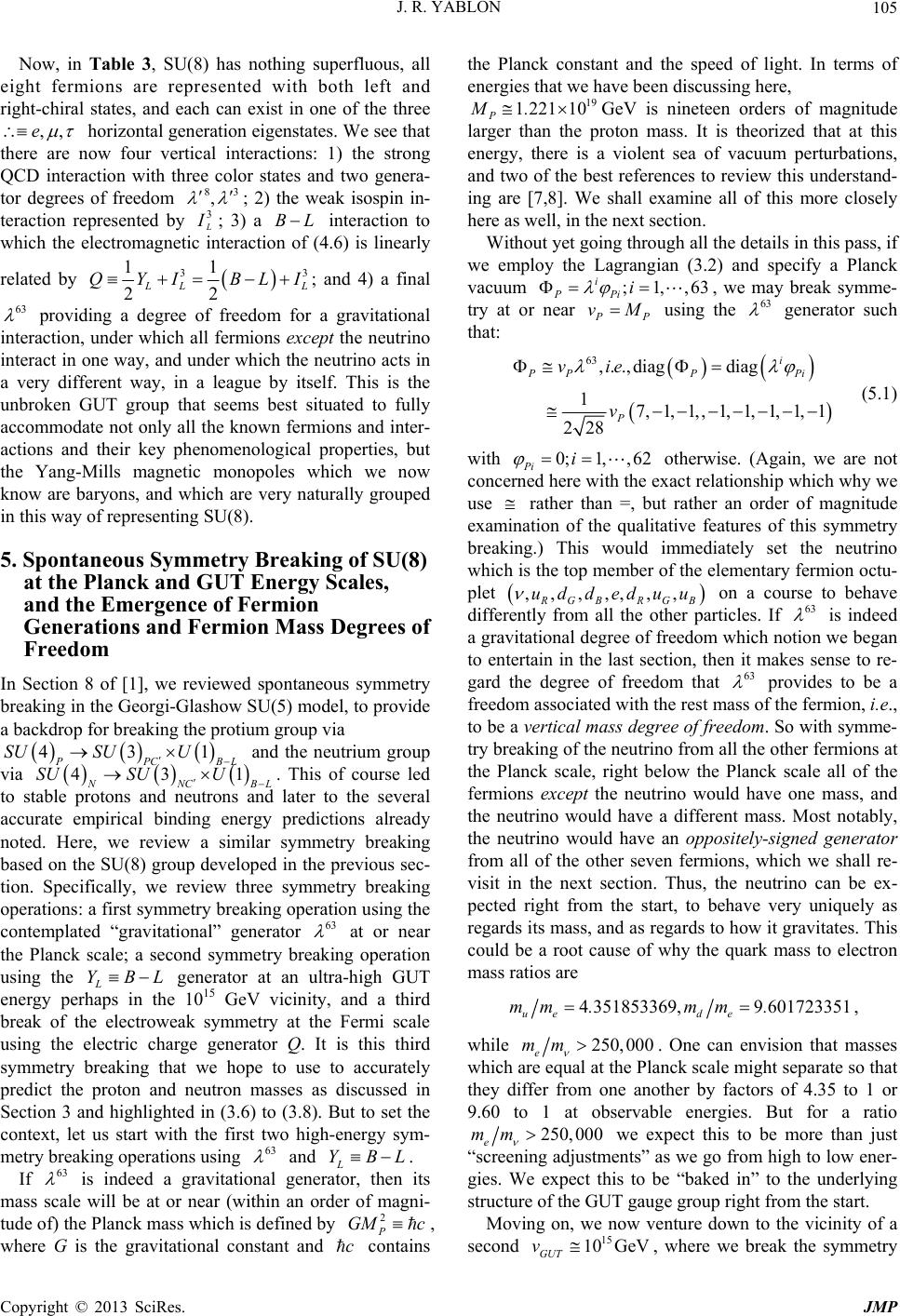 J. R. YABLON Copyright © 2013 SciRes. JMP 105 Now, in Table 3, SU(8) has nothing superfluous, all eight fermions are represented with both left and right-chiral states, and each can exist in one of the three ,,e horizontal generation eigenstates. We see that there are now four vertical interactions: 1) the strong QCD interaction with three color states and two genera- tor degrees of freedom 83 , ; 2) the weak isospin in- teraction represented by 3 ; 3) a BL interaction to which the electromagnetic interaction of (4.6) is linearly related by 33 11 22 LL QYIBLI; and 4) a final 63 providing a degree of freedom for a gravitational interaction, under which all fermions except the neutrino interact in one way, and under which the neutrino acts in a very different way, in a league by itself. This is the unbroken GUT group that seems best situated to fully accommodate not only all the known fermions and inter- actions and their key phenomenological properties, but the Yang-Mills magnetic monopoles which we now know are baryons, and which are very naturally grouped in this way of representing SU(8). 5. Spontaneous Symmetry Breaking of SU(8) at the Planck and GUT Energy Scales, and the Emergence of Fermion Generations and Fermion Mass Degrees of Freedom In Section 8 of [1], we reviewed spontaneous symmetry breaking in the Georgi-Glashow SU(5) model, to provide a backdrop for breaking the protium group via 431 PCB L SUSUU and the neutrium group via 431 NCB L SUSU U . This of course led to stable protons and neutrons and later to the several accurate empirical binding energy predictions already noted. Here, we review a similar symmetry breaking based on the SU(8) group developed in the previous sec- tion. Specifically, we review three symmetry breaking operations: a first symmetry breaking operation using the contemplated “gravitational” generator 63 at or near the Planck scale; a second symmetry breaking operation using the L YBL generator at an ultra-high GUT energy perhaps in the 1015 GeV vicinity, and a third break of the electroweak symmetry at the Fermi scale using the electric charge generator Q. It is this third symmetry breaking that we hope to use to accurately predict the proton and neutron masses as discussed in Section 3 and highlighted in (3.6) to (3.8). But to set the context, let us start with the first two high-energy sym- metry breaking operations using 63 and L YBL. If 63 is indeed a gravitational generator, then its mass scale will be at or near (within an order of magni- tude of) the Planck mass which is defined by 2 P GM c, where G is the gravitational constant and c contains the Planck constant and the speed of light. In terms of energies that we have been discussing here, 19 1 22110 P M. GeV is nineteen orders of magnitude larger than the proton mass. It is theorized that at this energy, there is a violent sea of vacuum perturbations, and two of the best references to review this understand- ing are [7,8]. We shall examine all of this more closely here as well, in the next section. Without yet going through all the details in this pass, if we employ the Lagrangian (3.2) and specify a Planck vacuum ;1,,63 i PPi i , we may break symme- try at or near P vM using the 63 generator such that: 63 , . .,diagdiag 17,1,1,,1,1,1,1,1 228 i PPP Pi P vie v (5.1) with 0;1,, 62 Pi i otherwise. (Again, we are not concerned here with the exact relationship which why we use rather than =, but rather an order of magnitude examination of the qualitative features of this symmetry breaking.) This would immediately set the neutrino which is the top member of the elementary fermion octu- plet ,,,,,,, GB RGB uddeduu on a course to behave differently from all the other particles. If 63 is indeed a gravitational degree of freedom which notion we began to entertain in the last section, then it makes sense to re- gard the degree of freedom that 63 provides to be a freedom associated with the rest mass of the fermion, i.e., to be a vertical mass degree of freedom. So with symme- try breaking of the neutrino from all the other fermions at the Planck scale, right below the Planck scale all of the fermions except the neutrino would have one mass, and the neutrino would have a different mass. Most notably, the neutrino would have an oppositely-signed generator from all of the other seven fermions, which we shall re- visit in the next section. Thus, the neutrino can be ex- pected right from the start, to behave very uniquely as regards its mass, and as regards to how it gravitates. This could be a root cause of why the quark mass to electron mass ratios are 4 351853369,9 601723351 ue de mm .mm . , while 250,000 e mm . One can envision that masses which are equal at the Planck scale might separate so that they differ from one another by factors of 4.35 to 1 or 9.60 to 1 at observable energies. But for a ratio 250,000 e mm we expect this to be more than just “screening adjustments” as we go from high to low ener- gies. We expect this to be “baked in” to the underlying structure of the GUT gauge group right from the start. Moving on, we now venture down to the vicinity of a second 15 10 GeV GUT v, where we break the symmetry  J. R. YABLON Copyright © 2013 SciRes. JMP 106 with L YBL. Again, we are simply for the moment talking about orders of magnitude for this energy scale. In fact, we have already discussed BL symmetry breaking at some length in Section 8 of [1]. But in that earlier discussion, we regarded 4 SU and 4 SU as disjoint groups each breaking down via 431, 431 PCB L NCB L SUSU U SUSU U to produce a 111 π3π1π1 CBB SUU U homotopy group with stable magnetic monopoles, essen- tially based on the disjointed groups of Table 1. Now, in contrast, we have conjoined these groups into SU(8) as represented by Table 2 above. So the symmetry breaking we are about to explore is a “wholesale” breaking of 4 SU and 4 SU together at once in SU(8), ver- sus the parallel, but “retail” symmetry breaking of 4 SU and 4 SU conducted in Section 8 of [1]. It is also worth noting as reviewed in Section 8 of [1], that Georgi and Glashow also break symmetry using the Y generator, albeit such that 11111 diagdiag, , ,, 33322 i iGUT Tv for a right-chiral quintuplet ,,,, RGBC C ddde v of fermions. So here, we are doing exact same thing as Georgi and Glashow insofar as using a Y generator to break the GUT symmetry circa 1015 GeV, but we are merely using a different group SU(8) versus SU(5), with all the fermions in the fundamental representation as shown in Table 2. Now let’s proceed. The group is now SU(8). Exactly as in (8.1) of [1], the vacuum we use is: GUTGUTGUT L vBLvY (5.2) Here, however, because of the SU(8) group, we have: L diag 111 111 diag 1,,,,1,,, 333 333 diag diag GUT i iGUT GUT GUT Tv vBLvY (5.3) Unlike Section 8 of [1], we no longer have 15 8 3 BL from which we set 15 2 23GUT v and so obtain the Clebsch-Gordon coefficient via 22 22 15 8 3GUT GUT vCv . Rather, here we have a BL specified in (4.2) which is a linear combination of five generators. Thus, to break symmetry here, picking off the coefficients in (4.2), we now must set: 63 4835 24 15 4443 ;;; 95 7321 22 2 ;2 35 3 GUTGUT GUT GUT GUT vvv vv (5.4) with all the remaining 0 i . The invariant scalar: 22222 63483524 15 2 222 1616 1634242 792181595 3 80 21 GUT GUT GUT v vCv (5.5) yields a Clebsch-Gordon coefficient 280 21 C (Note the 28 3 C from the earlier 15 8 3 BL included in the calculation of the above). One may then employ the procedure such as is outlined in (11.5) and (11.6) of [1] to obtain gauge bosons masses in the usual way, and these will have masses on the order of GUT v. But our interest here is in what happens at lower ener- gies, after this symmetry has been broken, because that brings us into energy ranges with are experimentally ob- servable. First, by breaking symmetry via GUTGUT L vBLvY , which for which the generator eigenvalues are 111 111 1,,,,1,,, 333 333 , we “fracture” the eight fermions in Tables 2 and 3 into a 1 L YBL hypercharge doublet of leptons ,e and a 1 3 L YBL hypercharge sextuplet of quarks ,, ,, RGBRG B duu udd. Of course, we know that ,, GB duu is a proton and ,, GB udd is a neutron, so this sextuplet may also be viewed as a 1 L YBL proton/neutron doublet ,pn . Referring to Tables 2 and 3, the weak isospin for each doublet ,, ,epn is given by 311 , 22 I . Of course for the proton this is arrived at by adding 31 111 2 222 I for its three quarks, and for the neutron similarly via 31111 2 222 I . 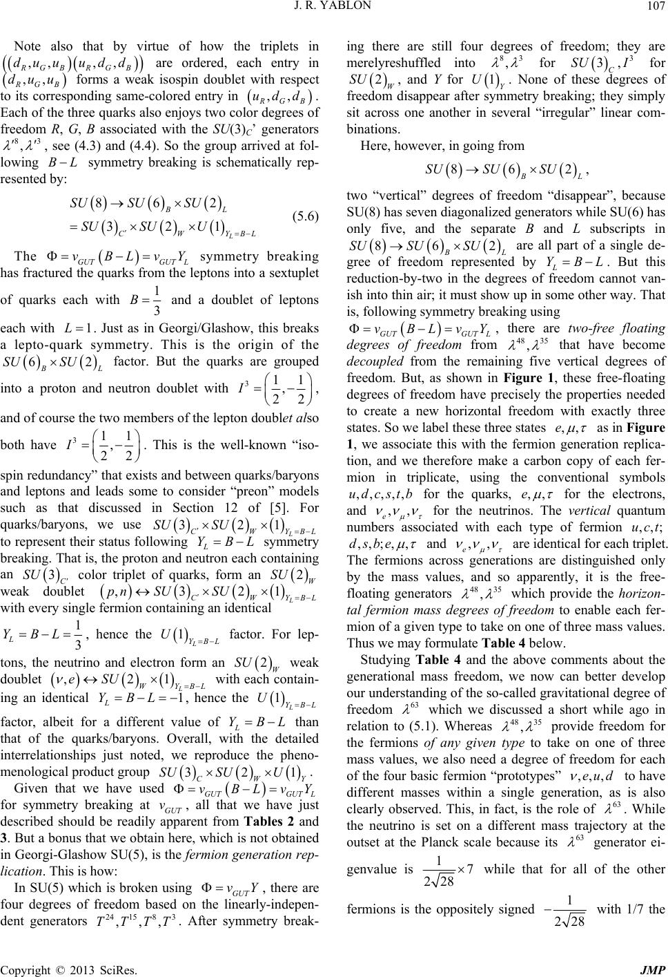 J. R. YABLON Copyright © 2013 SciRes. JMP 107 Note also that by virtue of how the triplets in ,, ,, RGBRG B duu udd are ordered, each entry in ,, GB duu forms a weak isospin doublet with respect to its corresponding same-colored entry in ,, GB udd . Each of the three quarks also enjoys two color degrees of freedom R, G, B associated with the SU(3)C’ generators 83 , , see (4.3) and (4.4). So the group arrived at fol- lowing BL symmetry breaking is schematically rep- resented by: 862 321 L BL CWYBL SUSU SU SUSU U (5.6) The GUTGUT L vBLvY symmetry breaking has fractured the quarks from the leptons into a sextuplet of quarks each with 1 3 B and a doublet of leptons each with 1L. Just as in Georgi/Glashow, this breaks a lepto-quark symmetry. This is the origin of the 62 L SU SU factor. But the quarks are grouped into a proton and neutron doublet with 311 , 22 I , and of course the two members of the lepton doublet also both have 311 , 22 I . This is the well-known “iso- spin redundancy” that exists and between quarks/baryons and leptons and leads some to consider “preon” models such as that discussed in Section 12 of [5]. For quarks/baryons, we use 321 L CWYBL SUSU to represent their status following L YBL symmetry breaking. That is, the proton and neutron each containing an 3C SU color triplet of quarks, form an 2W SU weak doublet ,321 L CWYBL pn SUSU with every single fermion containing an identical 1 3 L YBL, hence the 1L YBL U factor. For lep- tons, the neutrino and electron form an 2W SU weak doublet ,21 L WYBL eSU with each contain- ing an identical 1 L YBL, hence the 1L YBL U factor, albeit for a different value of L YBL than that of the quarks/baryons. Overall, with the detailed interrelationships just noted, we reproduce the pheno- menological product group 321 CWY SU SUU . Given that we have used GUTGUT L vBLvY for symmetry breaking at GUT v, all that we have just described should be readily apparent from Tables 2 and 3. But a bonus that we obtain here, which is not obtained in Georgi-Glashow SU(5), is the fermion generation rep- lication. This is how: In SU(5) which is broken using GUT vY , there are four degrees of freedom based on the linearly-indepen- dent generators 24 15 83 ,,,TTTT . After symmetry break- ing there are still four degrees of freedom; they are merelyreshuffled into 83 , for 3 3, C SUI for 2W SU , and Y for 1Y U. None of these degrees of freedom disappear after symmetry breaking; they simply sit across one another in several “irregular” linear com- binations. Here, however, in going from 862 L SUSU SU, two “vertical” degrees of freedom “disappear”, because SU(8) has seven diagonalized generators while SU(6) has only five, and the separate B and L subscripts in 862 L SUSU SU are all part of a single de- gree of freedom represented by L YBL. But this reduction-by-two in the degrees of freedom cannot van- ish into thin air; it must show up in some other way. That is, following symmetry breaking using GUTGUT L vBLvY , there are two-free floating degrees of freedom from 48 35 , that have become decoupled from the remaining five vertical degrees of freedom. But, as shown in Figure 1, these free-floating degrees of freedom have precisely the properties needed to create a new horizontal freedom with exactly three states. So we label these three states ,,e as in Figure 1, we associate this with the fermion generation replica- tion, and we therefore make a carbon copy of each fer- mion in triplicate, using the conventional symbols ,,,,,udcstb for the quarks, ,,e for the electrons, and ,, e for the neutrinos. The vertical quantum numbers associated with each type of fermion ,,;uct ,,;, ,dsbe and ,, e are identical for each triplet. The fermions across generations are distinguished only by the mass values, and so apparently, it is the free- floating generators 4835 , which provide the horizon- tal fermion mass degrees of freedom to enable each fer- mion of a given type to take on one of three mass values. Thus we may formulate Table 4 below. Studying Table 4 and the above comments about the generational mass freedom, we now can better develop our understanding of the so-called gravitational degree of freedom 63 which we discussed a short while ago in relation to (5.1). Whereas 48 35 , provide freedom for the fermions of any given type to take on one of three mass values, we also need a degree of freedom for each of the four basic fermion “prototypes” ,,,eu d to have different masses within a single generation, as is also clearly observed. This, in fact, is the role of 63 . While the neutrino is set on a different mass trajectory at the outset at the Planck scale because its 63 generator ei- genvalue is 17 228 while that for all of the other fermions is the oppositely signed 1 228 with 1/7 the 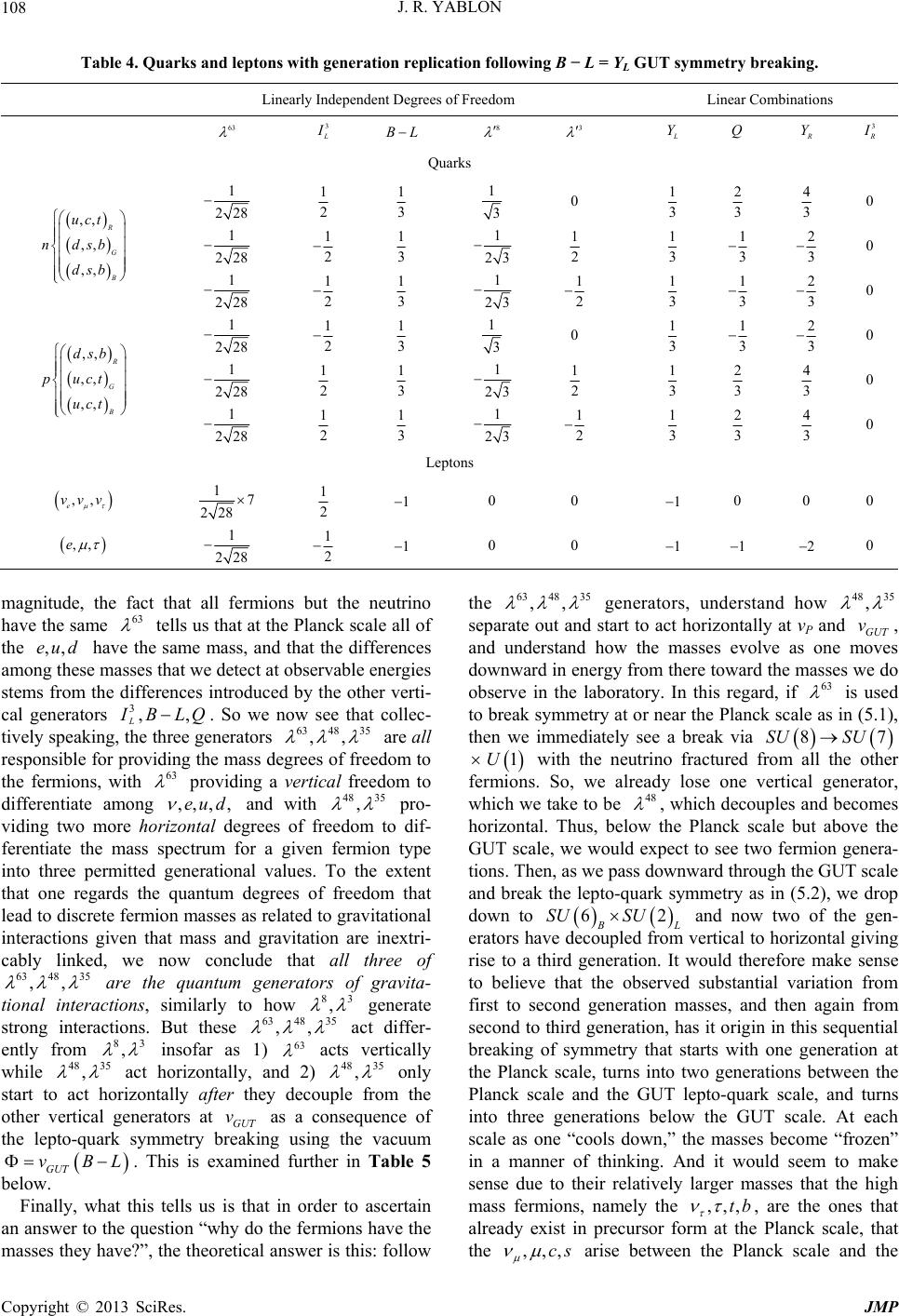 J. R. YABLON Copyright © 2013 SciRes. JMP 108 Table 4. Quarks and leptons with generation replication following B − L = YL GUT symmetry breaking. Linearly Independent Degrees of Freedom Linear Combinations 63 3 L 8 3 Y Q Y 3 Quarks 1 228 1 2 1 3 1 3 0 1 3 2 3 4 3 0 1 228 1 2 1 3 1 23 1 2 1 3 1 3 2 3 0 ,, ,, ,, R G B uct ndsb dsb 1 228 1 2 1 3 1 23 1 2 1 3 1 3 2 3 0 1 228 1 2 1 3 1 3 0 1 3 1 3 2 3 0 1 228 1 2 1 3 1 23 1 2 1 3 2 3 4 3 0 ,, ,, ,, R G B dsb puct uct 1 228 1 2 1 3 1 23 1 2 1 3 2 3 4 3 0 Leptons ,, e vvv 17 228 1 2 1 0 0 1 0 0 0 ,,e 1 228 1 2 1 0 0 1 1 2 0 magnitude, the fact that all fermions but the neutrino have the same 63 tells us that at the Planck scale all of the ,,eud have the same mass, and that the differences among these masses that we detect at observable energies stems from the differences introduced by the other verti- cal generators 3,, L BLQ. So we now see that collec- tively speaking, the three generators 6348 35 ,, are all responsible for providing the mass degrees of freedom to the fermions, with 63 providing a vertical freedom to differentiate among ,,,,eu d and with 4835 , pro- viding two more horizontal degrees of freedom to dif- ferentiate the mass spectrum for a given fermion type into three permitted generational values. To the extent that one regards the quantum degrees of freedom that lead to discrete fermion masses as related to gravitational interactions given that mass and gravitation are inextri- cably linked, we now conclude that all three of 63 4835 ,, are the quantum generators of gravita- tional interactions, similarly to how 83 , generate strong interactions. But these 63 48 35 ,, act differ- ently from 83 , insofar as 1) 63 acts vertically while 48 35 , act horizontally, and 2) 48 35 , only start to act horizontally after they decouple from the other vertical generators at GUT v as a consequence of the lepto-quark symmetry breaking using the vacuum GUT vBL . This is examined further in Table 5 below. Finally, what this tells us is that in order to ascertain an answer to the question “why do the fermions have the masses they have?”, the theoretical answer is this: follow the 6348 35 ,, generators, understand how 48 35 , separate out and start to act horizontally at vP and GUT v, and understand how the masses evolve as one moves downward in energy from there toward the masses we do observe in the laboratory. In this regard, if 63 is used to break symmetry at or near the Planck scale as in (5.1), then we immediately see a break via 87SU SU 1U with the neutrino fractured from all the other fermions. So, we already lose one vertical generator, which we take to be 48 , which decouples and becomes horizontal. Thus, below the Planck scale but above the GUT scale, we would expect to see two fermion genera- tions. Then, as we pass downward through the GUT scale and break the lepto-quark symmetry as in (5.2), we drop down to 62 L SU SU and now two of the gen- erators have decoupled from vertical to horizontal giving rise to a third generation. It would therefore make sense to believe that the observed substantial variation from first to second generation masses, and then again from second to third generation, has it origin in this sequential breaking of symmetry that starts with one generation at the Planck scale, turns into two generations between the Planck scale and the GUT lepto-quark scale, and turns into three generations below the GUT scale. At each scale as one “cools down,” the masses become “frozen” in a manner of thinking. And it would seem to make sense due to their relatively larger masses that the high mass fermions, namely the ,,,tb , are the ones that already exist in precursor form at the Planck scale, that the ,,,cs arise between the Planck scale and the 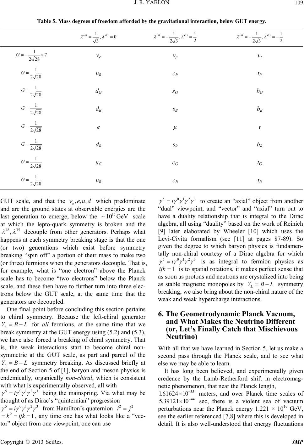 J. R. YABLON Copyright © 2013 SciRes. JMP 109 Table 5. Mass degrees of freedom afforded by the gravitational interaction, below GUT energy. 48 35 1,0 3 48 35 11 ,2 23 48 35 11 ,2 23 17 228 G νe νμ ντ 1 228 G uR cR tR 1 228 G dG sG bG 1 228 G dB sB bB 1 228 G e μ τ 1 228 G dR sR bR 1 228 G uG cG tG 1 228 G uB cB tB GUT scale, and that the ,,, eeu d which predominate and are the ground states at observable energies are the last generation to emerge, below the 15 ~10 GeV scale at which the lepto-quark symmetry is broken and the 48 35 , decouple from other generators. Perhaps what happens at each symmetry breaking stage is that the one (or two) generations which exist before symmetry breaking “spin off” a portion of their mass to make two (or three) fermions when the generators decouple. That is, for example, what is “one electron” above the Planck scale has to become “two electrons” below the Planck scale, and these then have to further turn into three elec- trons below the GUT scale, at the same time that the generators are decoupled. One final point before concluding this section pertains to chiral symmetry. Because the left-chiral generator L YBL for all fermions, at the same time that we break symmetry at the GUT energy using (5.2) and (5.3), we have also forced a breaking of chiral symmetry. That is, the weak interactions start to become chiral non- symmetric at the GUT scale, as part and parcel of the L YBL symmetry breaking. As discussed briefly at the end of Section 5 of [1], baryon and meson physics is endemically, organically non-chiral, which is consistent with what is experimentally observed, all with 50123 i being the mainspring. Via what may be thought of as Dirac’s “quinternian” progression 50123 i from Hamilton’s quaternion 22 ij 21kijk , any time one has what looks like a “vec- tor” object from one viewpoint, one can use 50123 i to create an “axial” object from another “dual” viewpoint, and “vector” and “axial” turn out to have a duality relationship that is integral to the Dirac algebra, all using “duality” based on the work of Reinich [9] later elaborated by Wheeler [10] which uses the Levi-Civita formalism (see [11] at pages 87-89). So given the degree to which baryon physics is fundamen- tally non-chiral courtesy of a Dirac algebra for which 50123 i is as integral to fermion physics as 1ijk is to spatial rotations, it makes perfect sense that as soon as protons and neutrons are crystalized into being as stable magnetic monopoles by L YBL symmetry breaking, we also bring about the non-chiral nature of the weak and weak hypercharge interactions. 6. The Geometrodynamic Planck Vacuum, and What Makes the Neutrino Different (or, Let’s Finally Catch that Mischievous Neutrino) With all that we have learned in Section 5, let us make a second pass through the Planck scale, and to see what else we may be able to learn. It has long been believed, and experimentally given credence by the Lamb-Retherford shift in electromag- netic phenomenon, that near the Planck length, 35 1.61624 10 meters, and over Planck time scales of 44 5.39121 10 sec, there is a violent sea of vacuum perturbations near the Planck energy 1.221 × 10¹⁹ GeV, see the earlier referenced [7,8] where this is developed in detail. It is also well-understood that energy fluctuations  J. R. YABLON Copyright © 2013 SciRes. JMP 110 of this magnitude on such a small scale do have the effect of topologically creating microscopic black holes, also called wormholes, with a Schwarzschild radius at or near the Planck length. Let us now take a closer look at ex- actly what is believed to occur at this scale. Again, along the lines discussed in Section 2, it is unlikely that humans will ever be able to directly observe physics at the Planck length, but the development of such physics in the con- text of a GUT may lead us to low energy mass and en- ergy predictions which—if they accord with empirical data—could then give us some confidence that the GUT which leads to such accord is also describing the Planck-length physics “behind the veil” with some sem- blance of accuracy. When Wheeler talks in his seminal work [8] about the geometrodynamic Planck vacuum, the vacuum he envi- sions is constructed from a series of simple algebraic calculations with which it is important to be familiar. So let us review those here. First, Newton’s law of gravita- tion 2 12 Gm mr contains a numerator 12 Gm m which has the same dimensions as the natural constant c. So the Planck mass 2 is defined as the unique, natural mass unit formed out of the Newtonian numerator from G, and c, namely: 2 P GM c. (6.1) The above means that P cG so that the Planck energy 25 PP EMc cG. The Fermi vev energy vF is similarly defined using the Fermi constant via 24 2FF Gv cc, with the 2 having historical origins based on how G was first defined before electroweak interactions were well-understood. Comparing “apples to apples” the correspondence is 2 GG. The reduced Compton wavelength of a Planck mass (6.1) is easily calculated to be: 3 PP G Mc c . (6.2) Now we consider a large collection of Planck masses separated from one another by , in what would be a natural state of resonance. The negative gravitational potential energy EG between any two separated by is easily calculated to be: 25 P GP PP GM cc EE G . (6.3) But this is simply the negative of the Planck energy! So as Wheeler first surmised, a collection of Planck mass fluctuations (on average) separated by the Planck length (on average) averages out to be a vacuum because the negative gravitational energy precisely cancels the posi- tive Planck energies which are posited in the first place, on average. Nonetheless, in very localized regions on the order of , there are very violent fluctuations of very high energy occurring. This is the so-called “geometro- dynamic vacuum.” It is also important to note that the Schwarzschild “black hole” radius for a (non-rotating) Planck mass may be calculated to be: 22 3 2222 P SP GM Gc G rG cc c . (6.4) Because the black hole radius is twice as large as the Planck length, this means that all of these fluctuations are occurring out of sight, behind a black hole horizon. On top of this, Hawking [12] teaches seventeen years after Wheeler’s initial elaboration of the geometrody- namic vacuum, based on general relativistic gravitational theory, that black holes emit a blackbody radiation spec- trum. So if we recognize that the Planck vacuum is a vacuum in which the masses on average are Planck masses separated on average by the Planck length, and then like any good student of statistics we ask the natural follow up question “what is the actual statistical distribu- tion of these energies about the average?” Hawking pro- vides a clear answer: because these fluctuations are oc- curring behind an event horizon, the distribution is ob- served externally to the event horizon as a thermody- namic, blackbody spectrum. It would also make sense, therefore, to consider the prospect that when we observe blackbody radiation in the natural world, we are in fact observing a gravitational phenomenon from the Planck vacuum screened through over twenty orders of magni- tude, which would render the blackbody spectrum that kicked off the quantum revolution in 1901 [13], a cones- quence of gravitational theory. So much for disunion between gravitational theory and quantum theory! But returning to GUTs, the Wheeler vacuum also teaches us something about the generator 63 with 63 1 diag7, 1, 1, 1, 1, 1,1,1 228 which we are associating on a preliminary basis with gravitation, which is this: One may look at the Planck vacuum in one of two entirely equivalent ways: First, one can say that there are a tremendous number of fluctua- tions with positive energy E on average, separated by on average, thus giving rise to an equal amount of negative gravitational energies E on average, thus resulting in a vacuum on average, which has a gravita- tional blackbody distribution of energy when viewed from outside the event horizon, and which is redshifted as our observational perch recedes to that from which Planck first characterized this distribution. Second, one can start with negative energy fluctuations, separate them by , and they will gravitate to produce positive en- ergy fluctuations. Each way of looking at this is equally  J. R. YABLON Copyright © 2013 SciRes. JMP 111 valid. It is a “chicken and the egg” question. One can develop an equally sensible description of the exact same physics no matter where one starts: positive Planck masses producing negative gravitational energies, or negative Planck masses producing positive gravitational energies. It does not matter. These are two alternative descriptions of exactly the same thing. Now, let’s talk about specific fermions, such as the ,,,,,,, GB RGB uddeduu of our SU(8) GUT group. How do these actually take root in the vacuum? How are they “conceived” and “born”? Through the lens of 1957, referring to electromagnetic charge Q, Wheeler says in [8] that “classical charge appears as the flux of lines of force trapped in a multiply connected metric ... trapped by the topology of the space.” In other words, charge gets “trapped” in the black hole wormholes. Updating this with all that we have learned in the intervening half cen- tury especially about Yang-Mills gauge theories and how charges such as the electric charge arise from the gen- erators of Yang-Mills theory, we might say that these Planck-mass fluctuations “trap” the Yang-Mills internal symmetries (which include the electric charge), and that this is how particles are “born.” Or, in parlance we in- troduce here, the physical fermions ,,,,,, GB R udded , GB uu arise when a Planck-scale fluctuation is “fertile- ized” by the Yang-Mills generators of internal symmetry. So a neutrino is conceived when a fluctuation with Planck mass magnitude is fertilized by the generator ei- genvalues in Table 2 corresponding to the neutrino. The same holds true for the up quark (in three colors), the down quark (in three colors) and the electron. Then, as Wheeler points out, the particles we observe from 20 orders of magnitude lower, have had all but the most miniscule portion of their original ~MP masses can- celled/averaged out by the positive and negative energy fluctuations of the vacuum, leaving behind only a small mass residue which results from the trapping of the field lines, i.e., from the fertilization. Those are the particles and masses we observe. But if the Planck vacuum raises a chicken and the egg question, the next question is this: how does nature de- cide whether the egg comes first or the chicken comes first? Does nature fertilize the positive energy fluctua- tions into observed particles, or the negative energy ones? Or, might she fertilize both? And what would a fertilized positive energy fluctuation look like, versus a fertilized negative energy fluctuation? And, fundamentally, how is this precisely-balanced positive versus negative energy symmetry in the Planck vacuum broken, in favor of the very miniscule (relative to the Planck vacuum) prepon- derance of positive energy over negative energy that we observe in the material universe? Now our 63 1 diag7, 1, 1, 1, 1, 1, 1, 1 228 generator provides the critical clue: If this is a gravita- tional generator as we have begun to surmise, and if this generator is actually used to break symmetry at or near the Planck energy as in (5.1), and given that this is the energy at which gravitation is dominant as is clear from (6.1) through (6.4), then this generator will have a great deal to do with how the Planck vacuum first gets fertile- ized to produce what we observe. So the gravitational charge of the neutrino being of opposite sign from the gravitational charges of all the other fermions suggests that perhaps neutrinos are fertilized negative energy Planck vacuum fluctuations and the up and down quarks and the electron are all fertilized positive energy Planck vacuum fluctuations. Not only would this neatly resolve the chicken and egg problem, but it would explain many other things as well, especially about the ever-elusive neutrino. First, this would truly place neutrinos in a class by themselves. They would be born of negative energy Planck scale fluctuations, brought about via the gravita- tional interactions of positive energy Planck scale fluc- tuations. Other fermions are rooted in “Planck matter”; neutrinos are rooted in “Planck gravitation.” Second, above the Planck energy, behind the event horizon, we would expect there to be a complete symmetry among all of the octuplet members ,,,,,,, GB RGB uddeduu . Any one fermion can readily decay into any other, and all would exist in equal numbers as part of an octuplet set. Thus, any time there is a neutrino, there are also seven other fermions to go along with that neutrino. Then, after we break the symmetry and the neutrino hooks up with negative energy fluctuations and the other seven fer- mions hook up with positive energy fluctuations, we would have a seven-to-one ratio of fermions which are rooted in positive energy fluctuations over fermions rooted in negative energy fluctuations. So as we reached lower and lower energies, there would be a net domi- nance of positive energy-rooted fermions over negative energy-rooted fermions. As such, this could help to ex- plain how the positive versus negative energy symmetry of the Planck vacuum becomes broken. This is especially so given the fact that at low energies the neutrino masses become so very much smaller than all the other fermion masses. Third, while we conventionally hold to the view that all matter gravitates the same way as all other matter, this would tell us that this conventional wisdom holds true for all matter except the neutrino. Below the Planck scale, the neutrino would fundamentally be a fermion rooted in negative energy fluctuations, while all of the other fer- mions would be rooted in positive energy fluctuations. This could certainly provide some degree of confidence that as we start to trace the development of the fermions from the Planck scale down to the laboratory scale, we  J. R. YABLON Copyright © 2013 SciRes. JMP 112 may come to understand why 4 351853369 ue mm . and 9 601723351 de mm ., while 250,000 e mm . The neutrino would start off in the Planck vacuum with a negative energy ~P M where represents the alteration in energy due to the fertilization of the negative energy gravitational fluctuation, while all the other fer- mions f would start off with a positive energy ~ f M rooted in the matter fluctuations. Then, after screening of twenty orders of magnitude, the neu- trino mass would end up very close to, and slightly larger than zero, and the rest of the fermion masses would end up more substantially above zero, with the observed masses between 5 2.5 10 and 6 2.5 10 times as large as what is observed for the neutrino. Further, if the neutrino gravitates differently from every other fermion (which we shall explore even further in the next section), then its elusive, idiosyncratic be- haveiors may be much better understood. From a tech- nology viewpoint, this also suggests that if one ever hopes to develop technologies to “shield” gravitation or overcome gravitational attraction other than by the brute force of rocket propulsion, the neutrino would be central to that undertaking. Harvesting and controlling the elu- sive neutrino, however, would be the core technology challenge. And, since neutrinos do exist throughout the universe as elusive as they may be, this would also mean that cosmological theories based on the supposition that all matter gravitates in relation to all other matter in exactly the same way would have to be modified to rec- ognize that the neutrino defies this supposition. As a consequence of the forgoing, let us now choose a negative gravitational charge for the neutrino to go with the negative energy fluctuations, as a matter of conven- tion. Then, let us introduce the hypothesis—which needs to be borne out through detailed calculation of its cones- quences—that the neutrinos are in fact conceived at or near the Planck scale when negative energy gravitational fluctuations in the Planck vacuum become fertilized with the negative gravitational charge of the neutrino 63 17 228 , and that quarks and electrons are born at or near the Planck scale when positive energy gravitational fluctuations in the Planck vacuum become fertilized with the positive gravitational charge of a quark or an electron 63 1 ,, 228 ude . And in this regard, choosing the convention of a nega- tive gravitational charge for the neutrino to go with the negative Planck energy fluctuations, we now explicitly define a gravitational interaction generator: 63 1 ;diag 7,1,1,1,1,1,1,1 228 GG . (6.5) We may find occasion to adjust this coefficient 1 228 as we calculate from this point forward, but this sign reversal, and the identification of 63 with a gravitational generator G, makes clear 1) that the neu- trino is understood to gravitate differently than all the other fermions as we shall further examine in a moment, and 2) that the neutrino is rooted in negative energy Planck fluctuations while all the other fermions are rooted in positive fluctuations. Or, as Wheeler might say, the neu- trino lines of force are trapped in negative energy topo- logical wormholes, and the quark and electron lines of force are trapped in positive energy topological wormholes. 7. Spontaneous Symmetry Breaking, Fermion and Generator Fractures, and Intergenerational Cabibbo Mixing of Left-Chiral Hypercharge Doublets As we now return to spontaneous symmetry breaking, it will be important to develop an understanding of what we shall call “fermion fractures” and “generator frac- tures.” While the fermion fracturing we are about to de- scribe may already be implicitly understood as a feature a spontaneous symmetry breaking, it is important to make this understanding explicit, as this will play a crucial role in understanding generation replication, and especially, the Cabibbo mixing which for leptons leads to so-called neutrino oscillations (which have been largely response- ble for demonstrating that the neutrino does have some tiny mass, contrary to what may have been believed two or three decades ago). When a gauge group has not been broken at all, and assuming that fermions have been assigned to the fun- damental representation of that gauge group, then any one fermion is completely free to decay into any other fermion. SU(3)QCD provides a good example of this. As we can see from Table 1, or as will be understood in any event, there are three color eigenstates 838 3 111 ,0, ,2 323 RG , 83 11 ,2 23 B . The symmetry is not broken, so any of these eigen- states may freely decay into any other one of these ei- genstates, even though their quantum numbers are dif- ferent. For example, all three color states R, G, B have completely different 3 , namely, 311 0, , 22 , yet they freely transition among themselves, which is central to QCD interactions. Similarly, as just discussed, above the Planck scale any fermion may transition into any  J. R. YABLON Copyright © 2013 SciRes. JMP 113 other fermion. Once a symmetry is broken, however, some fermions become “fractured” from some other fermions, and they are forbidden from decaying into one another except un- der very limited conditions. It is these limited conditions which are of central interest in the discussion following. Let us first break the symmetry of SU(8) at the Planck scale using (5.1), which we recast in light of (6.5) as: ,.., diag diag 17,1,1,,1,1,1,1,1 228 PP i PPi P vGie v (7.1) What then happens? Of course, similarly to what was discussed in Section 8 of [1], the vacuum commutes such that ,0,1,,48 i Pi . It also self-commutes with G, that is, ,,0 PP GvGG . But our real interest here is to look at the fermions themselves. The neutrino, with 17 228 G ,becomes fractured from all the other fermions with 1 228 G, and can no longer decay into any of these other states via the generator G that was used to break the symmetry. It would be as if the red quarks in QCD were suddenly for- bidden from decaying into green or blue quarks—but of course they can do so because the QCD symmetry is never broken. If G is a gravitational generator, then the neutrino can no longer undergo a gravitational decay through G into any other fermion. What does that mean? The neutrino will no longer gravitate with any other fer- mion except for another neutrino! But—and this is criti- cal—it may still undergo other types of decay through the generators of other interactions. Let’s elaborate: If the neutrino is to decay into any other fermion after the symmetry is broken via (7.1), it must decay into a fermion via an interaction governed by an interaction generator other than 63 gravitation such that the fer- mion has the same charge value under that other inter- action generator as that of the neutrino. Referring to Table 2 to make this clear, this means that the neutrino still can undergo a 35 decay into a u quark because each has 35 0 . And it can still undergo a 3 decay into any up quark, because these and the neutrino all have 31 2 L I. Most importantly, as will become central in the discussion be- low, the neutrino can still undergo BLY decay into an electron because both the neu- trino and the electron have the same 1 L BLY and so form a doublet under BLY . This latter abil- ity for the neutrino and the electron to decay into one another as like-charge members of a 1 L BLY doublet, lasts until the electroweak symmetry is finally broken at much lower (Fermi vev) energies into the elec- tromagnetic interaction. Now let’s look at the remaining seven fermions. Even after the symmetry breaking (7.1), these fermions are completely free to decay into one another via the gravi- tational generator G, because they are all like-valued 1 228 G eigenstates of G. They all continue to gravitate with one another, while the neutrino steps aside and stops gravitating with them. Indeed, starting at the Planck scale, and until one drops down to GUT energies on the order of 1015 GeV, these seven other fermions remain part of an SU(7) septuplet. Since all of these fer- mions are united by the common characteristic that they are born through the fertilization of positive (+) energy vacuum fluctuations, we shall refer to this group as SU(7)+. Thus, between the Planck scale and the GUT scale, the gauge group is 71 G SU U , and the topologically-stable SU(7) magnetic monopoles with all the fermions of a 2H atom are 111 π(7) π(1)π(1) GG SU UU . The 1G U emanates from the commutation of ,,0 PP GvGG , and is based on a neutrino singlet 17 228 G plus a septuplet of the remaining fermions all of which are in 1 228 G states. Again, importantly, the neutrino can no longer interact gravitationally via 63 with any of the remain- ing seven fermions. If it is to interact with them, it must do so via other non-gravitational interactions. Now let’s progress down the energy scale and break symmetry with BLY in the vicinity of 15 ~10 GeV GUT v using (5.2). The residual gauge groups are now those shown and discussed in (5.6), but let’s again look closely at how the fermions are fractured, and let’s also look at the loss of two generators going from 86SUSU. Referring now to Table 4, the 48 35 , generators are no longer in play as vertical generators, because two gen- erators are lost going from SU(8) to SU(6). These do not disappear entirely, but become horizontal as already dis- cussed, in a manner we shall momentarily develop fur- ther. As to the remaining five linearly-independent verti- cal generators in Table 4, the electrons and the quarks still remain a gravitational septuplet and so can still in- teract gravitationally with one another (while the neu- trino does not)! Following the rule that after symmetry  J. R. YABLON Copyright © 2013 SciRes. JMP 114 breaking the only decays which are permitted are decays under a given generator for which the decaying fermions have a like-charge, the remaining decays options are as among members of the quark sextuplet of fermions with 1 3 BL, and between the lepton doublet of fermions with 1BL . The former decays among fermions in the 1 3 BL sextuplet, consist of QCD strong interact- tions decays among the R, G, B color eigenstates based on the 83 , generators, and weak decays between states with 3 11 , 32 L L YI due to the common 1 3 L Y. The latter decays between the two fermions in the 1BL lepton doublet, consist of weak decays between the neutrino and the electron with 31 1, 2 L L YI due to the common 1 L Y . Now, however, most importantly, the quarks have be- come fully fractured from the leptons, and there is no more decay permitted between quarks and leptons. This is because, referring to Table 4, there is not a single ver- tical generator other than 63 for which any quark shares the same charge as any lepton, so hereafter, the only way for a quark to interact with a lepton is gravita- tionally. And the neutrino—the odd man out—does not interact gravitationally with any other fermions besides another neutrino, because its gravitational charge is dif- ferent from that of all the other fermions and that gravi- tational generator was used to break the Planck symmetry. Further, as was developed in detail in Section 8 of [1], the breaking of BL also creates stable magnetic monopoles 111 π3π1π1 CBB SUU U which manifest as protons and neutrons forming ,pn doublets with 1B. So this is also the symmetry break at which protons and neutrons are born. And, with BLY , as noted at the end of Section 5, the weak interaction becomes non-chiral to go along the with chiral non-symmetry of baryon interactions as discussed in Section 5 of [1]. So the BL symmetry breaking is responsible for several interrelated phenomena: it brings about the three generations observed at low energy, it brings about pro- tons and neutrons, it forecloses lepto-quark decays, and because BLY , it brings about the broken chiral symmetry of the weak interactions. Now, at some level, everything discussed so far in this section about fermion fracturing due to symmetry break- ing restates what is likely obvious, because it is known that one of the very basic consequences of symmetry breaking is that it forecloses certain decays which are permitted to occur in the higher state of symmetry before the symmetry is broken. From a thermodynamic view, it “freezes out” certain transitions below a certain critical temperature (recognizing too that some symmetries are not broken but are actually restored on the opposite end of the scale, near absolute zero, where electrons are su- perconducted freely without any apparent friction from the protons and neutrons from which they separate at GUT energies, which suggests that superconductivity may well be a phenomenon at which the SU(7) symmetry between electrons and quarks is restored so electrons can flow through rather than a round protons and neutrons). But the reason for focusing on fermion fracturing in this way, is because we will now venture into the not-obvious realm of generation replication and apply these observa- tions to understand what happens there as well. If the rule is that after symmetry breaking fermions can only decay into other fermions with like-charges under some interaction that was not used to break the symmetry, then what happens to the horizontal genera- tors 48 35 , after BLY symmetry breaking? Not only have quarks become fractured from leptons, but 48 35 , have themselves become fractured from the other generators! So we not only have fermion fracturing, we have generator fracturing. If we follow suit, then it would seem that a similar set of rules may well apply. Let’s explore. First, referring to Table 2, 48 1 diag0,6, 1, 1, 1,1,1, 1 221 and 35 1 diag0,0,5, 1,1,1,1, 1 215 are the two fractured generators. Because these no longer differentiate an observable vertical symmetry, but still do provide two degrees of freedom as illustrated in Figure 1 in section 5, let us transform these two generators into 48 35 , with the eigenvalues shown in Figure 1. No new calculation is required: we simply use (4.3) and (4.4) but without 8 and 3 , and so redefine 48 35 , 48 35 , according to: 48 483524 72 2 315 35 , (7.2) 353524 32 55 . (7.3) It is readily seen that 48 1 diag0, 2,1,1, 0, 0,0,0 23 and 35 1 diag0, 0,1,1, 0,0,0, 0 2 .  J. R. YABLON Copyright © 2013 SciRes. JMP 115 So these generators now do yield the SU(3) configure- tion shown in Figure 1, albeit with eight eigenstates, five of which are all zero-valued and trivial, and three of which are not. We can now label these three non-trivial eigenstates as: 48 35 1,0 3 e , (7.4) 48 35 11 ,2 23 , (7.5) 48 35 11 ,2 23 , (7.6) just as illustrated in Figure 1. However, these are now free-floating generators once the BLY symmetry is broken, so they no longer provide vertical symmetry quantum numbers for any of the fermions, as illustrated in Tables 3 and 4. Rather, they appear to provide a repli- cation of each fermion into three generations. But if this is the case, then they should lead to other facets of gen- eration replication as well, including Cabibbo-type mix- ing, and to the observation that the only way a particle from one generation can transform into a particle of an- other generation is via left-chiral weak interaction decays from one weak isospin to a different weak isospin, and not directly. As we shall now see, this is a consequence of the fermion and generator fracturing highlighted above and the “freezing” restrictions that come into play after symmetry breaking. Because the generators 4835 , have become frac- tured from the other generators, and given what we know about the fermion generations from experimental obser- vations, it appears that each of the ,,e eigenstates is fractured from one another so that it is now forbidden for a direct transition to take place between any of the three states (7.4), (7.5), (7.6), i.e., no decays may take place any longer via the 48 35 , (or 48 35 , ) interaction generators. Symbolically, e . Any decays that do take place, must occur via another generator for which the charges are the same as among the fermions involved in the decay. The fermion has to find a “loop- hole.” This is exactly like the discussion we had at the beginning of this section about the neutrino in relation to the remaining fermions from which it becomes fractured at v, or the fracturing of the quarks from the leptons at GUT v. In order to undergo decay into a different fermion, a fermion must find a different generator and a different fermion which has the same charge as the original fer- mion with respect to that different generator. So referring to Table 4, if a first-generation e fermion is to decay into a second generation μ fermion or a third-generation τ fermion, it must to do so via a genera- tor other than 48 35 , , into a fermion for which it shares an identical charge for that other generator. For the leptons, this is straightforward: the electron and the neutrino share a common charge 1 L BLY , and so for a first generation electron to become a second generation electron, it must go from e or e e , all of which have the same BL Y 1 . This is the only remaining “decay loophole.” Again this is exactly what was discussed earlier with regard to fermion fracturing. And so, for the first time, we see Cabibbo mixing and neutrino oscillations, be- cause that is exactly how these work as well. This also explains flavor non-conservation as regards the genera- tions: at the end of e or e e , what started as a first generation electron is now a second generation electron and neither 48 nor 35 is con- served, and this is because the generators are fractured. For the quarks it is a little more complicated, because this transition rule needs to be strengthened due to strong interactions. In particular, if a fermion can undergo a e transition by decay through at least one generator that is the same for both, then, for example, referring to Table 4, one could observe a G uc transition, because both the u and the G c have the same 1 3 L BL Y . This would imply that Cabibbo mixing can occur not only via weak but also via strong interactions, and the latter, of course, is not observed. So for horizontal symmetry transitions, it appears that we have to tighten the rules even further. Specifically, it appears that for a horizontal transition to be permitted, not just one, but all of the vertical degrees of freedom in Tables 3 and 4 must be the same as between the two fer- mions involved in the decay. Table 3 actually illustrates this rule the best, because this rule says that a horizontal e transition must occur either as a transition between the first and fifth, second and sixth, third and seventh, or fourth and eighth fermions in Table 3. These are the fermion doublets which share a common: 83 ,1,0,0,1 L eBL Y , (7.7) 83 111 ,,,0, 33 3 RR L ud BLY , (7.8) 83 , 1111 ,,,, 323 23 GG L ud BL Y (7.9) 83 , 11 11 ,,,. 323 23 BB L ud BL Y (7.10) So in sum, one can have neither e , nor e , nor uct , nor dsb tran-  J. R. YABLON Copyright © 2013 SciRes. JMP 116 sitions, because each of these has different 4835 , eigenvalues. These states are all fractured from one an- other. One cannot have intergenerational transitions be- tween ,e and any of the quark doublets because these have been fractured from one another by BL breaking. One cannot have intergenerational RG B transitions among (7.8), (7.9) and (7.10) because although QCD is never broken, the QCD generators are different as among red, green and blue states. If any ver- tical generators, or any horizontal generators are dif- ferent as between two fermions, then based on what we observe, the apparent rule is that the horizontal transi- tion is not permitted. So all that is permitted—the only “loophole” left for decay—are the e , , RG udu G d and B ud transitions, because these are the only transitions for which all of the generators listed are the same for both fermions. And here, because of the tightened rules when it comes to horizontal transitions based on fractured generators, even the right-chiral gen- erator Y is excluded, because this too is not the same as between the members of each of the above doublets. This is why we show Y in the above but not Y. This means only the left-chiral states may participate in tran- sitions among the e states in (7.4) to (7.6). Observationally, we know that this is also a characteristic of left-chiral weak generational interactions. These stronger rules for the horizontal generators may at first seem arbitrary, but they are not. They may be un- derstood because for the horizontal generators, not only are some fermions fractured from other fermions, but the horizontal generators themselves are fractured from the vertical generators. It is the fracturing of both generators and fermions which leads to such stringency. So for a vertical generator that breaks symmetry but is not itself fractured from the other vertical generators, transitions are permitted so long as at least one other vertical gen- erator provides the same charge as between the two tran- sition states. But for a generator which has itself been fractured from the other generators, the rule is even more restrictive. Now, transitions are permitted only if all of the involved vertical generators provide the same charge as between the two transition states. Now, the astute reader may notice that the electric charge Q and left-chiral weak isospin 3 are also not the same as between the two fermions in any of the dou- blets in (7.7) through (7.10) above. ,0,1Qe and 21 ,, 33 Qud as between the members of these doublets, as well as 311 ,, 22 L Ie and 311 ,, 22 L Iud . And so, the question might be asked, why are even these interactions permitted? After all, this changes the generators also, so by these rules, shouldn’t this be forbidden also? But further reflection makes this answer clear: the electric charge does not emerge as a physically-preclusive generator until it is used to break the electroweak symmetry at much lower energies determined by the Fermi vacuum F v 246.219651 GeV . This is the same way in which BL is not a preclusive generator until its breaks symmetry at GUT energies. So indeed, once we break electroweak symmetry, no transitions are permitted between genera- tions. But at the same time, neiter will e or ud be permitted, but this is because weak interact- tions are no longer permitted either (in the historical sense that the weak interaction becomes “weak”). So what we learn from this, is that the ability of fermions to change generations will wax and wane in lock step with the weak interaction itself and the breaking of elec- troweak symmetry, just as is observed! By imposing the more stringent rule that once the 48 35 , interaction generators have become fractured from the other generators by BL symmetry breaking at 15 ~10 GeV GUT v, no horizontal transitions are permit- ted among the (7.4) to (7.6) states unless all of the re- maining vertical generators—chiral symmetric or not— are the same as between the fermions involved in the transition, we arrive at precisely the type of mixing that is observed in nature as among the three generations. This makes generation mixing part and parcel of weak interactions, while excluding the strong interactions and even the right-chiral states from participation in genera- tional mixing. So, now we take the final, formal steps to mathemati- cally represent all of these decay restrictions. Referring to Section 12.12 of [14], the two generators 48 35 , introduce two degrees of freedom and so define three- non-trivial horizontal eigenstates ,,e in (7.4) through (7.6) and Figure 1, representing eigenstates of SU(3), which states are precluded from direct transformation into one another according to the rules just outlined be- cause they are fractured generators. SU(3) can be used to form unitary matrices U with 933 components. Because the only permitted transitions are (7.7) through (7.10), we can alter the phase of any of the 23 6 quark states which we designate ,ud ,,, ,,uctdsb following Table 3, without altering the physics. Similarly for leptons. But one may omit an overall phase change which still leaves the physics in- variant. This means that U must be a function of 933 minus 623 plus 1 parameters, i.e., 4 pa- rameters. But an orthogonal 33 matrix only has 3, 23C real parameters, which leaves one residual phase. So for the leptons l, we may choose to form this matrix in the representation:  J. R. YABLON Copyright © 2013 SciRes. JMP 117 111 1313 22 1133121232312323 223312123 23123 23 1000100 000 ee 000e0e e iδiδ l iiδiδ ll csc scss Ucssc cssccccssccssc scscss csccscsscc (7.11) and for the quarks q we form the analogous: 111 1313 22 1133121232312323 223312123 23123 23 1000100 000 ee 000e0e e iδiδ q iiδiδ qq cscscss Ucssc cssccccssccssc scscss csccscsscc (7.12) To implement the lepton mixing, we keep in mind from (7.7) that for a e transition to take place which alters the quantum numbers in (7.4) through (7.6), we cannot go directly from e , but must engage in a vertical transition between the states ,e in which all of the generators 8 1, 0,BL 30,1 L Y do not change. The only permitted tran- sition is e . Now, one can always apply (7.11) to both of ,e , but then one of them can always be transformed into a pure state while the other is similarly transformed, without changing the physics. In other words, all that is observable is the relative transition as between ,e . So following the usual conventions, we use (7.11) to transform the lower members of the ,e doublet, that is, we define: 113 13 12123 23123 23 12123 2312323 ee ee iδiδ ili iδiδ l ec scss e esccccssccsscUe sscs cc scsscc (7.13) Similarly for the quarks of each color C = R, G, B, we define: 11313 12123 2312323 12123 23123 23 ee ee C C iδiδ CiCCqCi iδiδ C C q dc scssd dssccccss ccsscsUd bsscsccscssccb (7.14) Because Y is not the same as between the members of each of the (7.7) through (7.10) doublets, right-chiral transitions are also precluded, and the only permitted transitions are for left-chiral states. So these will be pro- jected with 5 11 2 . Further, because 83 , are not the same except as between members of the four distinct doublets in (7.7) through (7.10), the only permitted tran- sitions will be between one lepton and another lepton, and between a first quark of a given color and a second quark of the same color ,,CRGB. This keeps the strong QCD interaction out of generation-changing tran- sitions (and also out of any CP violation), and makes this an exclusively weak, left-handed chiral phenomenon. So for leptons, the transition currents will be: 11313 5 12123 23123 23 12123 23123 23 55 1 ee1 2 ee 11 11 22 iδiδ le iδiδ l il iiiiLiL csc sse Jsccccssccssc sscscc scs scc Ue ee (7.14) And for quarks of each color ,,CRGB, they will be: 11313 5 12123 23123 23 12123 23123 23 55 1 ee1 2 ee 11 11 22 C iδiδ qCCC C iδiδ C q iCqiC iCiC iLC iLC csc ssd uctsccccssccsscs scsccscssccb uUdudud (7.15)  J. R. YABLON Copyright © 2013 SciRes. JMP 118 This is exactly what the phenomenology demonstrates! So, returning to the question posed at the very outset of the discussion following Table 2, not only does SU(8) not provide too much freedom, but upon careful consid- eration and development, it provides exactly the right amount of freedom to explain the precisely observed fermion phenomenology of three generations. Further, by applying the rule that fermions which are fractured from one another after symmetry breaking cannot decay into one another except by a vertical interaction other than the vertical interaction that was used to break symmetry, and that decay with regards to a fractured generator which thereafter becomes a free-floating horizontal degree of freedom is only permitted between fermion eigenstates for which all of the surviving vertical generators are the same, we can use SU(8) to explain everything that we know about the qualitative features of the interactions we observe, from generation replication to weak chiral non-symmetry to Cabibbo mixing to the fact that this mixing occurs only via weak isospin decays between left-handed states. And in the process we have perhaps found that neutrinos do not gravitate with any fermions aside from other neutrinos, which is likely to be of tre- mendous consequence as this is better developed and understood and especially if it can ever be exploited. Before concluding this section, let us now return to the first three generators 63 4835 ,, of SU(8). Based on the earlier review of how 63 breaks symmetry near the gravitational Planck scale and sets the neutrino on a tra- jectory to have a mass orders of magnitude smaller than that of any other fermion; given how the 4835 , frac- ture from the other vertical generators and form the basis for two horizontal degrees of freedom that underlie three fermion generations in which one fermion is distin- guished from one another solely by mass and not by any other quantum numbers from a vertical degree of free- dom, and given that mass and gravitation are inextricably linked such that gravitation is the “mass interaction,” we now formally associate these three generators 63 48 ,, 35 with the gravitational interaction, at the elementary particle level, below the GUT energy. Using (7.4) to (7.6) and (6.5), we highlight this connection in Table 5 of Section 5. The horizontal degrees of freedom from 48 35 , which to enable the fermions in each generation to have distinct masses in relation to their counterparts in the other two generations are shown horizontally, while the vertical degree of freedom G enabling each fermion within a generation to have a distinct mass is shown ver- tically. Of course, with SU(3)C remaining unbroken, dif- ferent colors of the same flavor of quark within one gen- eration have the same mass. As noted earlier, using the notation, the vertical gravitational generator G does not distinguish the ,,ud e masses from one an- other within a generation. So at high energies, as noted, the fermions (other than neutrinos) within a generation all have the same mass. It is only through the stages of symmetry breaking and the remaining generators BL Y , 3 and Q, that the mass spectrum within a generation separates. This may be thought of as mass/ energy differences emanating from strong, weak, and electromagnetic interactions, i.e., one may regard quark masses to differ from electron masses because they are quarks not leptons, and up and down quark masses to differ because their weak isospins and electric charges are different. Gravitational generators provide the free- dom for these differences to occur. As to interactions, after all symmetry breaking in- cludeing electroweak symmetry breaking is completed, the seven generators of SU(3) now are allocated as fol- lows: three degrees of freedom go to gravitation in the form of 63 48 35 ,, , two degrees of freedom go to strong QCD interactions via 83 , , one degree of freedom goes to left-chiral weak interactions via 3 , and the final degree of freedom goes to electromagnetic in- teractions via Q. Seven linearly-independent degrees of freedom, and eight vertical fermion eigenstates, thus ac- count perfectly, with nothing missing and nothing super- fluous, for the observed phenomenology of the fermions and their interactions, including generation replication and Cabibbo mixing, left-chiral weak interactions, and the elusive and perhaps gravitationally-defiant behavior of the neutrino. 8. Summary and Conclusion We have in the foregoing focused on the breaking of symmetry at the Planck scale and the GUT scale, which, astronomical observation aside, is many orders of mag- nitude beyond what we may ever hope to observe di- rectly. The final stage of symmetry breaking is elec- troweak symmetry breaking at the Fermi vev F v 246.219651 GeV . This is in the realm of observation, and the generator used to break this symmetry is the electric charge generator Q. This final symmetry break gives rise to the electromagnetic interaction which dominates atomic and chemical structure and much of what is most directly observed in the natural world be- yond gravitational interactions. That is, beyond objects falling to earth and planets wandering the heavens along prescribed trajectories, electromagnetic phenomena in electromagnetic and chemical and atomic form are our first line of direct experience of the natural world. Our experience of nuclear phenomena—based on the protons and neutrons which come to life as stable magnetic monopoles at the GUT scale as has been reviewed here and in [1]—comes to us through the laboratory instru- mentation that we used to extend the range of our physi-  J. R. YABLON Copyright © 2013 SciRes. JMP 119 cal senses, and gives rise to the vast preponderance of the matter that populates and animates the universe. When we break the electroweak symmetry we make use of the electric charge generator (4.6), and analo- gously to (5.1) through (5.3), employ the Fermi vacuum: i FiFF vQ , (8.1) which specifically means that: diagdiag 211122 0,,,,1,,, diag 333 333 i FiF FF T vvQ (8.2) Picking off the coefficients from the generators in (4.6), for each non-zero component of the vacuum we then have: 48 3524 15 8 27 422 ;;; 33 35 315 22 2; 33 FFFF F FFFF vvv vv (8.3) which leads to: 22 222 483524 15 8 2 222 471642 8 4 939159533 16 3 FFFFF F FF v vCv (8.4) and consequently an electroweak Clebsch-Gordon coef- ficient: 4 3 C. (8.5) This is how the electroweak symmetry is broken for the SU(8) group that we have developed throughout this paper. This final symmetry break fractures all fermions of different electric charges from one another, and so precludes their decay into one another. Referring to Ta- ble 4, weak isospin transitions between up and down quarks with differing charges 21 ,, 33 Qud are now precluded, as are similar transitions between elec- trons and neutrinos with ,0,1Qe . This shuts down the weak interaction (in the historical view, renders it “weak”; in hindsight it is probably better called the “faint” interaction), and because weak isospin decays as reviewed in the last section are the only avenues permit- ted for generation-changing transitions, generational transitions also are turned off in lock step. The only tran- sitions still permitted after electroweak symmetry break- ing, given that Q is a vertical symmetry generator and so not subject to the very stringent rules laid out in the last section for horizontal transitions, are the vertical, color- changing R, G, B transitions of QCD, which are still al- lowed to occur because the quarks involved in these interactions are part of a triplet in which 1 3 BL is the same for each, and the QCD symmetry remains un- broken. That is, the only permitted decays once elec- troweak symmetry is broken, are decays along the BL generator for particles of like BL with un- broken 83 , generators, which, of course, are strong QCD interactions. With the exception of the RG B transitions of QCD, no fermion may transform into any other different type of fermion. Now, following three stages of symmetry breaking—at the Planck scale, the GUT scale and the Fermi scale—all of the fermions have become fractured from one another, generation transitions cease, and the particles are frozen into the configurations of our everyday experience. The SU(8) symmetry with seven generator degrees of free- dom that we started with in Table 2 still does exist, but it has become hidden and distorted behind twenty orders of magnitude of vacuum screening and three stages of symmetry breaking that have fractured neutrinos from the other fermions and broken off their gravitational communication, broken the Planck symmetry between positive and negative energy fluctuations, fractured quarks from leptons, fractured two generators from the remaining five to provide horizontal generational replica- tion, brought about Cabibbo-type mixing among these generations for left-handed chiral projections only, and finally, fractured the upper and lower members of the like-hypercharge YL (weak isospin) doublets from one another, turned off the weak interactions, and frozen the particles in place so that all we observe at the lowest en- ergies are electromagnetic and strong interactions, as well as the bulk interaction of gravitating masses which is eluded by the neutrino. This GUT, which is based on the hypothesis that bary- ons are Yang-Mills magnetic monopoles and is rooted in the SU(4)P and SU(4)N subgroups developed in Section 7 of [1] which yielded over half a dozen accurate predict- tions in [1,2] as reviewed in Section 1 here, leads system- atically to all of the qualitative particle and interaction phenomenology which we are able to observe with our senses and the extension of our senses through experi- mental apparatus. But the confirmation of the particular GUT proposed here, versus other possible GUTs which reproduce similar phenomenally, needs to come through mass and energy predictions which continue the suc- cessful empirical matches developed in [1,2]. As dis- cussed in Section 3, one would expect that these energy predictions should come about by developing the re- maining -containing terms in the Lagrangian density (3.2) which we have not yet developed, and then making  J. R. YABLON Copyright © 2013 SciRes. JMP 120 use of these to calculate various energies 3 dEx L to be matched up with empirical data. Along the way, the development should proceed on a parallel course to that of Sections 2 through 11 of [1], making use of the non-Abelian Klein-Gordon Equation (3.10), representing scalar sources as J , employing the same sort spin sums and the same Gaussian ansatz modeling of fer- mions that was developed respectively in Sections 3 and 9 of [1], and keeping in mind the clues we have elabo- rated in (3.6) through (3.8) and (3.11) here, all while em- ploying the GUT and symmetry breaking that has been elaborated here. It is clear from [1,2] that it will be possible via this ap- proach to calculate and predict definitive mass and en- ergy values, just as has been done previously in [1] and [2]. It will then be left to interpret those values as we did in Sections 11 and 12 of [1] and throughout [2], and to compare them with experimental data to try to ascertain the meaning of those calculations and predictions to ob- tain sensible numerical matches to observed energy data. That is, we clearly will be able to calculate energies. The question will be whether the energies we are able to cal- culate will match and make sense in relation to the em- pirical data as well as they did in [1,2]. Success in this endeavor, if it should arrive, would validate that this particular GUT may indeed be the one that nature has selected to govern the phenomenology of the material universe, and would provide some confi- dence that the development elaborated here does reach “behind the veil” to explain how nature really does oper- ate in energy domains likely to forever remain beyond the reach of our direct senses and the extension of our senses gained through experimental devices and meth- ods. REFERENCES [1] J. R. Yablon, “Why Baryons Are Yang-Mills Magnetic Monopoles,” Hadronic Journal, Vol. 35, No. 4, 2012, pp. 401-468. http://www.hadronicpress.com/issues/HJ/VOL35/HJ-35-4 .pdf [2] J. R. Yablon, “Predicting the Binding Energies of the 1s Nuclides with High Precision, Based on Baryons which are Yang-Mills Magnetic Monopoles,” Journal of Mod- ern Physics, Vol. 4 No. 4A, 2013, pp. 70-93. doi:10.4236/jmp.2013.44A010 [3] H. Georgi and S. Glashow, “Unity of All Elementary- Particle Forces,” Physical Review Letters, Vol. 32, 1974, p. 438. doi:10.1103/PhysRevLett.32.438 [4] http://5dstm.org/ [5] G. E. Volovok, “The Universe in a Helium Droplet,” Clarendon Press, Oxford, 2003. [6] J. Beringer, et al., (Particle Data Group), “PR D86, 010001,” 2012. http://pdg.lbl.gov/2012/listings/rpp2012-list-neutrino-pro p.pdf [7] C. W. Misner, K. S. Thorne and J. A. Wheeler, “Gravita- tion,” Freeman, New York, 1973, p. 1190. [8] J. A. Wheeler, “On the Nature of Quantum Geometrody- namics,” Annals of Physics, Vol. 2, 1957, pp. 604-614. doi:10.1016/0003-4916(57)90050-7 [9] G. Y. Reinich, “Electrodynamics in the General Relativity Theory,” Transactions of the American Mathematical So- ciety, Vol. 27, No. 1, 1925, pp. 106-136. doi:10.1090/S0002-9947-1925-1501302-6 [10] J. A. Wheeler, “Geometrodynamics,” Academic Press, Boston, 1962, pp. 225-253. [11] C. W. Misner, K. S. Thorne and J. A. Wheeler, “Gravita- tion,” W. H. Freeman & Co., New York, 1973. [12] S. W. Hawking, “Black Hole Explosions?” Nature, Vol. 248, No. 5443, 1974, pp. 30-31. doi:10.1038/248030a0 [13] M. Planck, “On the Law of Distribution of Energy in the Normal Spectrum,” Annalen der Physik, Vol. 4, 1901, p. 553. doi:10.1002/andp.19013090310 [14] F. Halzen and A. D. Martin, “Quarks and Leptons: An Introductory Course in Modern Particle Physics,” John Wiley & Sons, Hoboken, 1984.
|