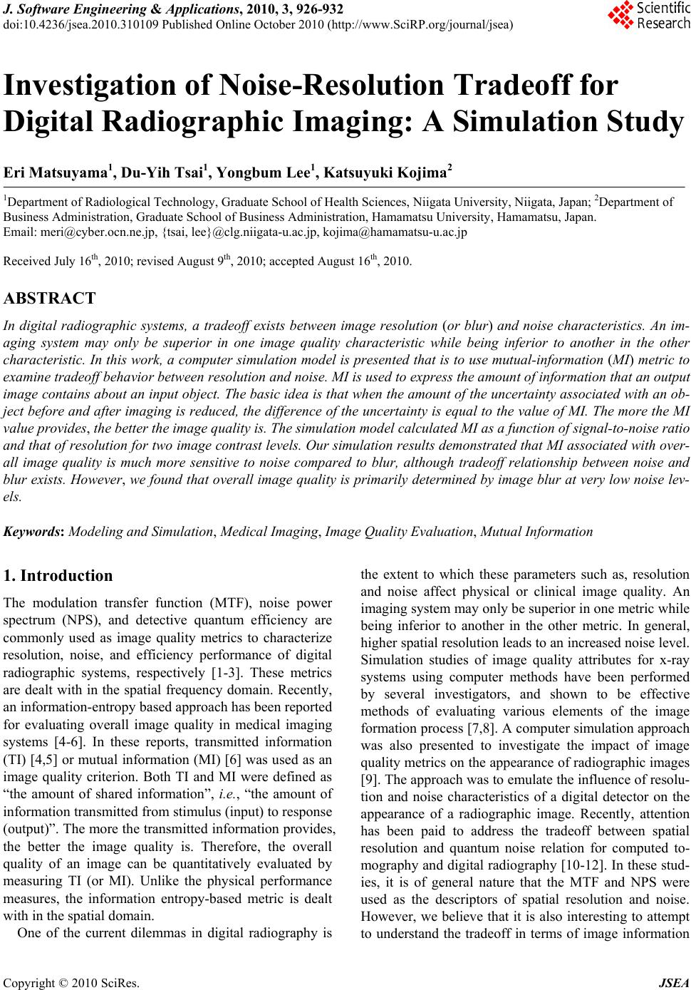J. Software Engi neeri n g & Applications, 2010, 3, 926-932
doi:10.4236/jsea.2010.310109 Published Online October 2010 (http://www.SciRP.org/journal/jsea)
Investigation of Noise-Resolution Tradeoff for
Digital Radiographic Imaging: A Simulation Study
Eri Matsuyama1, Du-Yih Tsai1, Yongbum Lee1, Katsuyuki Kojima2
1Department of Radiological Technology, Graduate School of Health Sciences, Niigata University, Niigata, Japan; 2Department of
Business Administration, Graduate School of Business Administration, Hamamatsu University, Hamamatsu, Japan.
Received July 16th, 2010; revised August 9th, 2010; accepted August 16th, 2010.
ABSTRACT
In digital radiographic systems, a tradeoff exists between image resolution (or blur) and noise characteristics. An im-
aging system may only be superior in one image quality characteristic while being inferior to another in the other
characteristic. In this work, a computer simulation model is presented that is to use mutual-information (MI) metric to
examine tradeoff behavior between resolution and noise. MI is used to express the amount of information that an output
image contains about an input object. The basic idea is that when the amount of the uncertainty associated with an ob-
ject before and after imaging is reduced, the difference of the uncertainty is equal to the value of MI. The more the MI
value provides, the better the image quality is. The simulation model calculated MI as a function of signal-to-noise ratio
and that of resolution for two image contrast levels. Our simulation results demonstrated that MI associated with over-
all image quality is much more sensitive to noise compared to blur, although tradeoff relationship between noise and
blur exists. However, we found that overall image quality is primarily determined by image blur at very low noise lev-
els.
Keywords: Modeling and Simulation, Medical Imaging, Image Quality Evaluation, Mutual Information
1. Introduction
The modulation transfer function (MTF), noise power
spectrum (NPS), and detective quantum efficiency are
commonly used as image quality metrics to characterize
resolution, noise, and efficiency performance of digital
radiographic systems, respectively [1-3]. These metrics
are dealt with in the spatial frequency domain. Recently,
an information-entropy based approach has been reported
for evaluating overall image quality in medical imaging
systems [4-6]. In these reports, transmitted information
(TI) [4,5] or mutual information (MI) [6] was used as an
image quality criterion. Both TI and MI were defined as
“the amount of shared information”, i.e., “the amount of
information transmitted from stimulus (input) to response
(output)”. The more the transmitted information provides,
the better the image quality is. Therefore, the overall
quality of an image can be quantitatively evaluated by
measuring TI (or MI). Unlike the physical performance
measures, the information entropy-based metric is dealt
with in the spatial domain.
One of the current dilemmas in digital radiography is
the extent to which these parameters such as, resolution
and noise affect physical or clinical image quality. An
imaging system may only be superior in one metric while
being inferior to another in the other metric. In general,
higher spatial resolution leads to an increased noise level.
Simulation studies of image quality attributes for x-ray
systems using computer methods have been performed
by several investigators, and shown to be effective
methods of evaluating various elements of the image
formation process [7,8]. A computer simulation approach
was also presented to investigate the impact of image
quality metrics on the appearance of radiographic images
[9]. The approach was to emulate the influence of resolu-
tion and noise characteristics of a digital detector on the
appearance of a radiographic image. Recently, attention
has been paid to address the tradeoff between spatial
resolution and quantum noise relation for computed to-
mography and digital radiography [10-12]. In these stud-
ies, it is of general nature that the MTF and NPS were
used as the descriptors of spatial resolution and noise.
However, we believe that it is also interesting to attempt
to understand the tradeoff in terms of image information

Investigation of Noise-Resolution Tradeoff for Digital Radiographic Imaging: A Simulation Study927
i
such as mutual information.
In this paper, a computer simulation approach is
presented that is to employ the MI metric to investigate
tradeoff behavior between resolution and noise. The
simulation model calculated MI as a function of signal-
to-noise ratio and that of resolution for two specific image
contrast levels. Two simulation studies were per- formed
separately; the first simulation was carried out to inves-
tigate the relationship between image blurring and MI for
various levels of noise, and the second simulation was
conducted to investigate the relationship between image
noise and MI for different extent of blurring. In this work,
a total of 2,688 simulations were performed in order to
conduct a detailed analysis and achieve a better under-
standing of noise-resolution tradeoff.
2. Theoretical Framework
MI is a concept from information theory [13,14] and is
also referred to as TI as described in the section of pre-
ceding Section [4-6]. MI has been applied in medical
image processing, particularly for image registration
[15-18]. The definition of the term of MI has been pre-
sented in various ways in the literature. We will briefly
describe MI, as used in the image evaluation sense, rather
than as used in the image registration sense.
Given events s1,….. sn occurring with probabilities p1,
p2, …….pn, the Shannon entropy H is defined as
12 2
1
(, ,...)log
n
ni
i
H
pp ppp


 (1)
Considering x and y as two random variables corre-
sponding to an input variable and an output variable, the
entropy for the input and that for the output are denoted
as H(x) and H(y), respectively. For this case, the MI can
be defined as
(;)()()() (
()()(, )
yx
)
M
IxyHxH xHyHy
Hx Hy Hxy
 
 (2)
where H(x,y) is the joint entropy, and Hx(y) and Hy(x) are
conditional entropies. The entropies and joint entropy are
given as
2
() log
i
i
i
H
xp
p (3)
2
() log
j
j
j
H
yp
p (4)
2
(, )log
ij ij
ij
H
xypp

(5)
where pi and pj are the marginal probabilities, and pij is
the joint probability.
A useful way of visualizing the relationship among
these entropies is provided by a Venn diagram as shown
in Figure 1. The MI measures how much the uncertainty
of input x is known if output y has been given. It can be
easily shown that if input and output are generally inde-
pendent, then H(x,y) = H(x) + H(y). Consequently, their
MI is zero (i.e., transmitted information is equal to zero).
In other words, observing y does not reduce the uncer-
tainty of x. If, however, x = y, i.e., H(x) = H(y), then MI =
H(x). Under this condition, the information about input x
can be obtained completely. We apply the MI measure to
evaluate image quality of digital radiography based on the
following reasoning. Consider an experiment in which
every input has a unique output belonging to one of the
various output categories. The inputs may be considered
to be a set of subjects, for example, a test sample object
with steps of various thickness, whereas the outputs may
be their corresponding images varying in optical density
or gray level. If the inputs can be recognized completely
when the outputs have shown, then the quality or the per-
formance of the transmission channel of the system (i.e.,
imaging system), can be perfect. In the cur- rent study, a
method of occurrence-frequency-based computation was
used for calculating the entropies of input, output, and
their joint entropies. The details of the calculation pro-
cedure can be found in the literature [4-6].
3. Methods
3.1. Computer Simulation
A simulation was designed, and its framework is as
follows. A simulation image g(x,y) was given by a spatial
convolution between a uniformly-distributed signal (an
object) f(x,y) having intrinsic noise u(x,y) and a blurring
function B. If the external noise v(x,y) was also taken into
consideration, the resulting image could be represented
by the following formula:



5
1
(, )(, )(, )
(, ),
s
g
xysf xyuxyWB
vxy K





(6)
H y ( x ) H x ( y )
MI ( x , y )
H ( x ; y )
H ( x ) H ( y )
Figure 1. The relations between conditional and joint en-
tropies, and the mutual information.

Investigation of Noise-Resolution Tradeoff for Digital Radiographic Imaging: A Simulation Study 928
where the symbol represents the convolution opera-
tion, and s is an integer representing the number of steps
of the simulated image. The terms of W and K are
weighting coefficients used to adjust noise level.

In the simulation studies, the input image f(x,y) was a
five-step wedge with a specific intensity or a pixel value
on each step. Both u(x,y) and v(x,y) were zero-mean
Gaussian noise with a standard deviation of 0.5. In the
studies, for simplicity, the term of v(x,y) × K was consid-
ered the external noise and is equal to the intrinsic noise
of u(x,y) × W (i.e., u(x,y) × W = v(x,y) × K). We used a
“m × m” (m is an odd integer) 8-neighborhood averaging
filter as the blurring function. The extent of blurring was
adjusted by varying the filter size (FS). The reason for
choosing neighborhood averaging filter was its ease of
implementation and effectiveness, which were confirmed
by experiments.
Two simulations were performed. The first simulation
was carried out to investigate the relationship between
image blur and MI for various noise levels at specific
image contrasts levels. In this study, we defined image
contrast as the difference of the mean pixel values
between two adjacent steps of a simulated step wedge.
We used signal-to-noise ratio (SNR) to describe the ex-
tent of noise level. Notice that the signal and noise used
for SNR calculation were f(x,y) and u(x,y) × W, respec-
tively, as given in Equation (6). In this work, combina-
tions of 64 various SNRs (range, 24-43 dB), 21 various
FSs (range, 3-41), and two different contrast levels (20
and 40) were used for simulation studies. As a result, a
total of 2688 simulations were performed for the analysis
of resolution-noise tradeoff.
The second simulation was performed to investigate
the relationship between image noise and MI for differ-
ent extent of blurring at specific image contrast levels.
3.2. Step-wedge Phantom Images
For verification and validation of our designed computer
simulation models, phantom images of an acrylic
step-wedge with 2, 4, 6, 8, and 10 mm in thickness were
obtained using the following exposure conditions. The
specific exposure factors were kept at 42 kV and 10 mA,
the focus-imaging distance was taken at 185 cm, and the
exposure time was varied ranging from 0.1 to 0.5 sec. An
imaging plate for computed radiography was used as a
detector to record x-ray intensities.
4. Simulation Results and Discussion
Figures 2 and 3 compare the computer-simulated images
versus the phantom images obtained. The simulated images
shown in the figures were generated using Equation (6).
A perceptual comparison of the simulated images and
phantom images indicates that these images were
(a) (b) (c)
(d) (e) (f)
Figure 2. Perceptual evaluation of computer simulated im-
ages. (a) Computer-simulated image. The parameters used
are: W = 130, SNR = 26.1 dB, contrast = 70, FS = 3. (b) The
magnified image from the rectangular area shown in (a). (c)
The magnified image from the rectangular area shown in
(b). (d) Step wedge phantom image. Exposure time was 0. 5 s.
The step wedge was placed 30 cm apart from the center
toward the cathode end for imaging. (e) The magnified im-
age from the rectangular area shown in (d). (f) The magni-
fied image from the rectangular area shown in (e).
(a) (b) (c)
(d) (e) (f)
Figure 3. Perceptual evaluation of computer simulated im-
ages. (a) Computer-simulated image. The parameters used
are: W = 300, SNR = 19.3 dB, contrast = 70, FS = 3. (b) The
magnified image from the rectangular area shown in (a). (c)
The magnified image from the rectangular area shown in
(b). (d) Step wedge phantom image. Exposure time was 0. 1 s.
The step wedge was placed 30 cm apart from the center
toward the cathode end for imaging. (e) The magnified im-
age from the rectangular area shown in (d). (f) The magni-
fied image from the rectangular area shown in (e).
very similar in appearance with respect to noise, blur and
visibility of detail. The comparison result indicated that
our designed mathematical model provides a good means
of simulating the resolution and noise characteristics of
digital radiographic systems.

Investigation of Noise-Resolution Tradeoff for Digital Radiographic Imaging: A Simulation Study929
Figure 4 illustrates MI as a function of FS for varying
levels of SNR ranging from 24 to 41 dB at an image con-
trast of 40. It should be noted that FS is associated with
the extent of blurring: the greater the FS value is, the
higher the extent of blurring becomes. As shown in Fig-
ure 4, MI decreases with the increase of FS (i.e., increase
of image blur) when noise levels are very low (i.e., high
SNR; for example, SNR>36 dB in this study), although
the decrease is relative small. This means that, in the case
of low noise levels, the effect of the level of blur on the
MI is not so obvious in comparison to noise.
When noise increases to medium levels (for example,
36 dB ≥ SNR ≥ 31 dB in this report), MI initially in-
creases with the increase of FS and then gradually de-
creases after reaching the maximum value. The increase
in MI value might be because that, in spite of deteriora-
tion of image resolution, the increase of FS could give
rise to a significant decrease of noise. Thus, MI is greatly
dependent on the decrease of noise level compared to the
deterioration of image resolution. However, on the
contrary, when FS increases to a certain level, the MI
value is greatly influenced by the deterioration of resolu-
tion as compared to that by the decrease of noise.
In the case of high noise levels (for example, SNR ≤
28 dB), MI increases gradually with the increase of FS
until reaching its maximum value. After that, MI value
showed insignificant decreasing. The reasoning could be
made as follows: 1) initially, the increase of FS might
result in a great decrease of noise, and this yields the
increase of MI, although the increase of FS itself might
give rise to a small decrease of MI. In other words, the
decrease of noise level dominated the variation of MI. 2)
However, when FS continued increasing, a tradeoff point
appeared. The location, indicated by an arrow on each
graph shown in Figure 4, was referred to as the tradeoff
point in this study. The location corresponds to the
maximum value of MI. For instance, the tradeoff points
for SNR = 41, 31, and 25 dB can be found at FS = 3, 9,
and 17, respectively. It is noted that, not surprisingly, the
location of the tradeoff point depends on SNR. An
oblique line in the figure depicts the trend in the change
of the location. As shown in the figure, MI reaches to its
maximum at a finer resolution when SNR increases.
Figure 5 plots MI as a function of FS for varying lev-
els of SNR at an image contrast of 20. Overall, the trend
of this case is similar to that at image contrast of 40. It
can be seen from Figures 4 and 5 that images with
higher contrast show greater MI values in comparison to
those with lower contrast, if both images have the same
spatial resolution (same FS) and the same noise level
(same SNR). It is reasonable to conclude that a higher
contrast image shows better image quality.
Figure 6 shows MI as a function of SNR for various
01 3 5 7 9111315 1719 21232527 29
1.0
1.2
1.4
1.6
1.8
2.0
2.2
FS (Filter Size)
MI (Mutual Information) [bits]
SNR24
SNR25
SNR26
SNR27
SNR28
SNR29
SNR30
SNR31
SNR32
SNR33
SNR36
SNR41
Figure 4. Relationship between FS and MI for varying lev-
els of SNR at an image contrast of 40.
01 35 7 911 13 1517 19 21 232527 29
0.6
0.8
1.0
1.2
1.4
1.6
1.8
2.0
2.2
FS
(
Filter Size
)
MI (Mutual Information) [bits]
SNR24
SNR25
SNR26
SNR27
SNR28
SNR29
SNR30
SNR31
SNR32
SNR33
SNR35
SNR36
SNR37
SNR39
SNR41
Figure 5. Relationship between FS and MI for varying lev-
els of SNR at an image contrast of 20.
sizes of FS at an image contrast of 40. The results
indicate that, basically, MI value increases with the in-
crease of SNR (decrease in noise level). The figure illus-
trates only the results covering a range of SNR from 29
to 36 dB, where intersections between the line graphs
occur. The intersection between two graphs indicates that
two images have the same overall image quality, al-
though the images may show different extent of blur. For
instance, the intersection between the graphs of FS = 3
and FS = 41 is located near SNR = 33. It is noted that an
image blurred by a smoothing filter of FS = 41 might
decrease the MI value because of resolution deterioration
caused by blurring. On the contrary, the MI value might
increase because of the decrease of noise resulting from
smoothing operation. This means that the physical
quality of an image is mutually adjusted by resolution

Investigation of Noise-Resolution Tradeoff for Digital Radiographic Imaging: A Simulation Study 930
and noise properties at a specific image contrast. The
result implies that the contribution of resolution attribute
and that of noise attribute to the MI value vary depending
on the levels of noise and blur. Here, it should be noted
that the external noise (i.e., the term of v(x,y) × K shown
in equation (6)) also served as a factor that influences
overall image quality of an image.
Figure 7 shows MI as a function of SNR for various
sizes of FS at image contrast of 20. The figure also
shows that the MI value increases with the increase of
SNR. From Figures 6 and 7, it is noted that the MI value
for the image with lower contrast is lower than that with
higher contrast. However, the trends of the two cases are
similar. As described earlier, a higher contrast image
shows better image quality compared to a lower contrast
image.
29 303132 33 34 35 36
1.7
1.8
1.9
2.0
2.1
2.2
2.3
SNR
(
Si
g
nal-to-Noise Ratio
)
[dB]
MI (Mutual Information) [bits]
FS 3
FS 5
FS 7
FS11
FS21
FS31
FS41
Figure 6. Relationship between SNR and MI for varying
sizes of FS at an image contrast of 40.
32 33 34353637 38 39 40
1.5
1.6
1.7
1.8
1.9
2.0
2.1
2.2
2.3
SNR
(
Si
g
nal-to-Noise Ratio
)
[dB]
MI (Mutual Information) [bits]
FS 3
FS 5
FS 7
FS11
FS21
FS31
FS41
Figure 7. Relationship between SNR and MI for varying
sizes of FS at an image contrast of 20.
Figures 8 and 9 show the MI values, plotted as a func-
tion of SNR and FS (blur) at image contrast of 40 and 20,
respectively. Figure 8 corresponds to Figures 4 and 6,
while Figure 9 corresponds to Figures 5 and 7. As
shown in the figures, MI reaches to the maximum value
when an image has very high SNR. Moreover, it is noted
that MI is much more sensitive to noise compared to blur.
It is also noted that the image with a higher contrast level
provides greater MI and shows better image quality in
comparison with that with lower contrast level, if the two
images have the same noise and blurring levels (Figures
8 and 9).
Figures 10 and 11 are plots of SNR (noise) versus FS
(blur) for four different MI values (i.e., 2.276, 2.206,
2.159, and 2.090), corresponding to four various trans-
mitted efficiency (i.e., 98%, 95%, 93%, and 90%) for the
Figure 8. MI calculated as a function of SNR and FS (blur)
at image contrast of 40.
Figure 9. MI calculated as a function of SNR and FS (blur)
at image contrast of 20.

Investigation of Noise-Resolution Tradeoff for Digital Radiographic Imaging: A Simulation Study931
1 510 15 20 25 30 35 40
32
33
34
35
36
37
38
39
40
41
42
FS (Filter Size)
SNR (Signal-to-Noise Ratio) [dB]
98% (MI=2.276)
95% (MI=2.206)
93% (MI=2.159)
90% (MI=2.090)
Figure 10. A plot of SNR versus FS for four different MI
values at an image contrast of 40.
1 510 15 2025 30 35 40
32
33
34
35
36
37
38
39
40
41
42
FS (Filter Size)
SNR (Signal-to-Noise Ratio) [dB]
98% (MI=2.276)
95% (MI=2.206)
93% (MI=2.159)
90% (MI=2.090)
Figure 11. A plot of SNR versus FS for four different MI
values at an image contrast of 20.
cases of contrast levels of 40 and 20, respectively. In this
study, “transmission efficiency” was used and defined as
the ratio between MI and the input entropy, i.e.,
η=(MI/H(x)) %. The efficiency η may also be used as a
measure for indicating how good the imaging quality of
an image receptor is. Points shown on each curve in the
figures, obtained from different combinations of SNR
and FS, have the same MI values, thus providing the
same overall image quality. It is observed that a mini-
mum point exists at each graph. Noted that only high
SNR levels (i.e., low noise level) ranging from 32 to 42
dB are depicted in Figures 10 and 11. Because the
minimum points for those SNR levels lower than 32 dB
did not appear in our simulation studies. As shown in the
two figures, tradeoff relationship between image noise
and blur exists on the right of the minimum point. This
means that a combination of a lower noise level and a
deteriorated resolution might provide the same physical
image quality as a combination of a higher noise level
and a higher resolution level. On the left of the minimum
point, however, image quality is primarily determined by
resolution when the SNR of an image is higher than 32
dB in our investigation. In other words, the image quality
of a very-low-noise image is almost determined by the
extent of blur, even when noise level had slight
variations. There might be two reasons for this. First, for
images of very low noise levels, image quality might not
be affected by small change of noise levels. As described
in the section of Theoretical Framework, MI measures
how much the uncertainty of input is known if output has
been given. As a result, very small changes in the amount
of noise might not influence the amount of the uncer-
tainty. Second, as shown in Figures 4 and 5, MI has a
significant increase with the increase of deterioration of
resolution at low FS values (range, 3-9 in the simulation
studies).
It must be addressed here that the purpose of this study
was to present a computer simulation approach to
investigate tradeoff behavior between resolution and
noise using the MI metric. In order to validate the results
obtained from this study, we will perform visual
evaluation and compare them in the future work.
Our simulation results showed that the proposed
simulation approach by employing mutual-information
metric to examine tradeoff behavior between resolution
and noise is useful, reliable and challenging.
5. Conclusions
A computer simulation study for examining resolution-
noise tradeoff behavior has been presented. In this study
MI was used as an image quality metric for the analysis.
Our simulation results demonstrated that the MI value
associated with overall image quality is much more sen-
sitive to noise compared to blur, although tradeoff rela-
tion between noise and blur exists. However, at very low
noise levels (SNR values higher than 32 dB), we found
that overall image quality is primarily determined by
image blur. However, a comparison between the result of
physical evaluation and that of perceptual evaluation was
not made in this work. It would be a very interesting re-
search question for our future study.
REFERENCES
[1] H. Fujita, K. Doi and M. L. Giger, “Investigation of Basic
Imaging Properties in Digital Radiography 6 MTFs of
II-TV Digital Imaging Systems,” Medical Physics, Vol.
12, No. 6, 1985, pp. 713-720.

Investigation of Noise-Resolution Tradeoff for Digital Radiographic Imaging: A Simulation Study 932
[2] M. L. Giger, K. Doi and H. Fujita, “Investigation of Basic
Imaging Properties in Digital Radiography 7 Noise Wie-
ner Spectra of II-TV Digital Imaging Systems,” Medical
Physics, Vol. 13, No. 2, 1986, pp. 131-138.
[3] A. Maidment and M. Yaffe, “Analysis of Spatial-Fre-
quency-Dependent DQE of Optically Coupled Digital
Mammography Detectors,” Medical Physics, Vol. 21, No.
6, 1994, pp. 721-729.
[4] E. Matsuyama, D. Y. Tsai, Y. Lee, M. Sekiya and K.
Kojima, “Physical Characterization of Digital Radiological
Images by Use of Transmitted Information Metric,” Pro-
ceedings of 2008 SPIE Medical Imaging, Vol. 6913, 2008,
pp. 69130V1-V8.
[5] D. Y. Tsai, Y. Lee and E. Matsuyama, “Information En-
tropy Measure for Evaluation of Image Quality,” Journal
of Digital Imaging, Vol. 21, No. 3, 2008, pp. 338-347.
[6] E. Matsuyama, D. Y. Tsai and Y. Lee, “Mutual Informa-
tion-Based Evaluation of Image Quality with Its Prelimi-
nary Application to Assessment of Medical Imaging Sys-
tems,” Journal of Electronic Imaging, Vol. 18, No. 3,
2009, pp. 033011-1-11.
[7] R. Nishikawa and S. Lee, “Preliminary Results on a
Method for Producing Simulated Mammograms,” pre-
sented at the AAPM 44th Annual Meeting, Montreal,
Quebec, Canada, 2002.
[8] A. Tingberg, C. Herrmann, J. Besjakov, A. Almen, P.
Sund, D. Adliene, S. Mattsson, L. Mansson and W. Pan-
zer, “What is Worse: Decreased Spatial Resolution or In-
creased Noise,” Proceedings of SPIE Medical Imaging,
Vol. 4686, 2002, pp. 338-346.
[9] R. S. Saunders Jr. and E. Samei, “A Method for Modify-
ing the Image Quality Parameters of Digital Radiographic
Images,” Medical Physics, Vol. 30, No. 11, 2003, pp. 3006-
3017.
[10] T. Fuchs and W. Kalender, “On the Correlation of Pixel
Noise, Spatial Resolution and Dose in Computed Tomo-
graphy,” Physica Medica, Vol. XIX, No. 2, 2003, pp. 153-
164.
[11] B. Li, G. B. Avinash and J. Hsieh, “Resolution and Noise
Trade-off Analysis for Volumetric CT,” Medical Physics,
Vol. 34, No. 10, 2007, pp. 3732-3738.
[12] A. R. Pineda and H. H. Barrett, “What Does DQE Say
about Lesion Detectability in Digital Radiography,” Pro-
ceedings of 2001 SPIE Medical Imaging, Vol. 4320, 2001,
pp. 561-569.
[13] C. E. Shannon, “Mathematical Theory of Communica-
tion,” Bell System Technology Journal, Vol. 27, 1948, pp.
379-423, pp. 623-656.
[14] C. E. Shannon and W. Weaver, “The Mathematical The-
ory of Communication,” The University of Illinois Press,
Urbana, 1948.
[15] D. Skerl, B. Likar and F. Pernus, “A Protocol for Evalua-
tion of Similarity Measures for Rigid Registration,” IEEE
Transactions on Medical Imaging, Vol. 25, No. 6, 2006,
pp. 779-791.
[16] G. D. Tourassi, B. Harrawood, S. Singh and J. Y. Lo,
“Information-Theoretic CAD System in Mammography:
Entropy-Based Indexing for Computational Efficiency
and Robust Performance,” Medical Physics, Vol. 34, No.
8, 2007, pp. 3193-3204.
[17] J. P. W. Pluim, J. B. A. Maintz amd M. A. Viergever,
“Mutual-Information-Based Registration of Medical Images:
A Survey,” IEEE Transactions on Medical Imaging, Vol.
22, No. 8, 2003, pp. 986-1004.
[18] G. D. Tourassi, E. D. Frederick, M. K. Marley and C. E.
Floyd Jr., “Application of the Mutual Information Crite-
rion for Feature Selection in Computer-Aided Diagnosis,”
Medical Physics, Vol. 28, No. 12, 2001, pp. 2394-2402.