Journal of Water Resource and Protection, 2013, 5, 395-404
http://dx.doi.org/10.4236/jwarp.2013.54039 Published Online April 2013 (http://www.scirp.org/journal/jwarp)
Coupling Singular Spectrum Analysis with Artificial
Neural Network to Improve Accuracy of Sediment
Load Prediction
Sokchhay Heng, Tadashi Suetsugi
Interdisciplinary Graduate School of Medicine and Engineering, University of Yamanashi, Kofu, Japan
Received January 8, 2013; revised February 19, 2013; accepted February 28, 2013
Copyright © 2013 Sokchhay Heng, Tadashi Suetsugi. This is an open access article distributed under the Creative Commons Attribu-
tion License, which permits unrestricted use, distribution, and reproduction in any medium, provided the original work is properly
cited.
ABSTRACT
Sediment load estimation is generally required for study and development of water resources system. In this regard,
artificial neural network (ANN) is the most widely used modeling tool especially in data-constraint regions. This re-
search attempts to combine SSA (singular spectrum analysis) with ANN, hereafter called SSA-ANN model, with ex-
pectation to improve the accuracy of sediment load predicted by the existing ANN approach. Two different catchments
located in the Lower Mekong Basin (LMB) were selected for the study and the model performance was measured by
several statistical indices. In comparing with ANN, the proposed SSA-ANN model shows its better performance re-
peatedly in both catchments. In validation stage, SSA-ANN is superior for larger Nash-Sutcliffe Efficiency about 24%
in Ban Nong Kiang catchment and 7% in Nam Mae Pun Luang catchment. Other statistical measures of SSA-ANN are
better than those of ANN as well. This improvement reveals the importance of SSA which filters noise containing in the
raw time series and transforms the original input data to be near normal distribution which is favorable to model simu-
lation. This coupled model is also recommended for the prediction of other water resources variables because extra in-
put data are not required. Only additional computation, time series decomposition, is needed. The proposed technique
could be potentially used to minimize the costly operation of sediment measurement in the LMB which is relatively rich
in hydrometeorological records.
Keywords: Artificial Neural Network; Singular Spectrum Analysis; Coupled Model; Sediment Load; Mekong Basin
1. Introduction
Quantification of sediment load is necessary for study
and development of water resources system such as res-
ervoir storage, dam, irrigation/navigation channel, soil
and water conservation measure, environmental impact
assessment, etc. [1-5]. Sediments are the end products of
land surface erosion governed mainly by hydrometeo-
rology, topography, geology and land use/cover [1,2].
Sediment data are lacking for rivers in many areas of the
world, especially in developing and remote regions [6].
However, it can be estimated with the aid of modeling
approaches. The hydrologic and terrain conditions of a
river basin change spatio-temporally and this causes dif-
ficulties in determining their effects on sediment erosion
and transport. This drawback has encouraged the appli-
cation of black box models, e.g. artificial neural network
(ANN). ANN forecasts outputs using experiences learned
from historical data. Its application can be found in many
sectors including finance, medicine, water resources, and
so forth. There are many types of ANN and the recog-
nized ones are feedforward, kohonen and hopfield net-
works [7]. In predicting and forecasting water resources
variables, feedforward networks are almost exclusively
applied [8]. The term “ANN” used in this paper is re-
ferred to feedforward artificial neural network.
The ANN model is commonly used in river basins
with data scarcity because it does not require detailed
physical information of the system. By just providing
hydrometeorogical information as inputs, ANN can pre-
dict sediment load at the watershed outlets with high ac-
curacy. Kisi and Shiri [5] applied ANNs to predict sus-
pended sediment concentration (SSC) in Eel River (USA)
with rainfall and discharge as inputs and obtained very
satisfactory results with Nash-Sutcliffe Efficiency (NSE)
between 0.80 and 0.84 in validation stage. Sediment
C
opyright © 2013 SciRes. JWARP

S. HENG, T. SUETSUGI 396
yield of various sub-watersheds in Kapgari River Basin
(India) is modeled well by ANN (input: rainfall and tem-
perature) with NSE ranging from 0.76 to 0.83 in vali-
dation stage [9]. In Pari River (Malaysia), ANNs (input:
discharge) perform very well in simulating suspended
sediment load (SSL) with NSE equal to 0.99 and 1.00 in
validation stage [10]. ANN can be employed also to ana-
lyze the hysteretic phenomenon of sediment transport
[11]. It is a very practical and promising modeling tool in
the context of sediment load prediction [12] and its out-
puts can be potentially used for design and management
purposes in water-related development projects [7].
Although ANN has been proved to perform well in
modeling sediment load and other hydrological variables,
many researches have been carried out further in order to
improve its accuracy by coupling with other methods.
Sediment load is generally predicted by using hydrome-
teorological variables and the most common of which are
rainfall and discharge. Naturally, the time series of such
variables are very noisy due to the effects of climate
variation and other human activities. Thus, one common
way to improve the prediction accuracy of ANN is to
perform some pre-processing of the inputs and this re-
quires another method. This kind of technique is known
as a coupled approach which has been getting more in-
terest recently. Kisi [13] developed a range-dependent
neural network (RDNN) for predicting sediment load at
two stations operated by the US Geological Survey.
RDNN splits the original data series into three ranges
which are afterward used as ANN inputs. In term of
model efficiency measured by determination coefficient
(R2), RDNN is slightly better than ANN for larger R2
about 0.5% at Santa Clara Station, and both models per-
form comparably at Calleguas Station. If considering
root mean square error (RMSE) and mean absolute error
(MAE), RDNN is much better than ANN at both stations.
Selection of a method for input pre-processing should
match ideally the specific learning problems. In this
study, singular spectrum analysis (SSA) was proposed
because it is generally seen as an adaptive noise-reduc-
tion algorithm [14]. SSA is a tool decomposing a time
series into a number of components with simple struc-
tures, which can be often identified as trends, seasonality
and other oscillatory series, or noise components, and it
does not require any statistical assumptions while per-
forming the analysis [15,16]. The application of SSA in
analyzing hydrometeorological time series (e.g. rainfall,
discharge, temperature) can be found in Hanson et al. [17]
and Marques et al. [18]. This method can be used par-
ticularly to extract the main components of rainfall and
discharge series and to provide good forecast for them
[18]. Sivapragasam et al. [14] combined SSA with the
support vector machine method (the latter called SSA-
SVM approach) to predict rainfall at Station 23 (Singa-
pore) and runoff from Tryggevælde catchment (Den-
mark), and the results were compared with those of the
non-linear prediction (NLP) method. For rainfall predic-
tion, SSA-SVM performs much better than NLP for less
RMSE 36% in calibration stage and 28% in validation
stage. For runoff prediction, SSA-SVM is also superior
to NLP for less RMSE 64% in calibration phase and 59%
in validation phase. To our knowledge, there are no any
studies associating SSA with ANN for predicting sedi-
ment load yet.
The present study attempts to combine SSA with ANN,
hereafter called SSA-ANN model, for sediment load pre-
diction with expectation to obtain more accurate results
than using ANN alone. The specific objectives are to
examine the application of the SSA-ANN model in pre-
dicting monthly average m and compare its
performance with that of the existing ANN approach.
The case study was firstly tried in Ban Nong Kiang
(BNK) catchment. In order to show consistency, another
case study was conducted in Nam Mae Pun Luang
(NMPL) catchment. Both catchments are located in the
Lower Mekong Basin (LMB).

SSL SSL
2. Materials and Methods
2.1. Study Catchments
The LMB is a trans-boundary river basin which partially
covers four Southeast Asian countries: Lao PDR, Thai-
land, Cambodia and Vietnam. This basin is relatively
rich in hydrometeorological records except sediment [19].
As illustrated in Figure 1, BNK catchment is located in
the western part of the basin and drains approximately
1405 km2. The elevation in this catchment decreases
from north to south and varies from just over 1300 m to
about 200 m. The average catchment slope is around
22.5%. Rainfall in this area is influenced by the south-
west monsoon (May-October) blowing from Bay of Ben-
gal bringing humid and hot weather. From November to
April, this period is known as dry season. Natural to-
pography and mountain ranges make this catchment ori-
ented in a leeward direction creating a rain shadow and
therefore little rainfall amount, about 1080 mm/year. The
annual discharge is 17.10 m3/s. Sediment yield in BNK
catchment is around 44 t/year/km2. The dominant land
use is tree cover or forest and the dominant soil type is
Orthic Acrisols.
Situated in the northwest of the LMB (Figure 1),
NMPL catchment has a drainage area of about 260 km2.
The feature of catchment topography is west-east gradi-
ent with elevation varying between 510 and 1670 m. The
average catchment slope is approximately 32.5%. This
catchment receives rainfall around 1950 mm annually
and produces an average discharge of 2.22 m3/s. Rainfall
pattern in this area is influenced by the southwest mon-

S. HENG, T. SUETSUGI 397
Figure 1. Map of the study catchments.
soon as well but the amount is much higher than that in
BNK catchment because NMPL catchment is oriented in
windward direction. Sediment yield of this catchment is
about 58 t/year/km2. The larger sediment yield can be
explained by topographic feature of each catchment. Mo-
saics and shrub cover dominates the land use in the
catchment and the dominant soil type is Orthic Acrisols.
Poor gauging stations in term of data availability and
completeness are commonly found in developing and re-
mote regions as located the LMB. These two catchments
were selected based on data availability: 20 years (1982-
2003, no data in 1986 and 1987) in BNK catchment and
22 years (1980-2001) in NMPL catchment.
2.2. Data
The main data used in this study are rainfall (R), dis-
charge (Q) and suspended sediment load (SSL). SS L is
the product of Q and SSC. The daily time series of R, Q
and SSC were obtained from Mekong River Commission.
R and Q series are continuous but SSC series are discon-
tinuous with few samples per month. The average sam-
pling frequency in BNK and NMPL catchment is about 2
and 4 samples per month, respectively. This provokes the
study in monthly basis. The monthly average SSL(SSLm)
is the product of monthly average Q(Qm) and monthly
average


SSC SSCQ
mm

and Rm (monthly average
rainfall) were employed as inputs for model calculation
and SSLm was used for comparison with the model out-
puts. Due to data limitation, the model inputs consist of
only Rm and Qm. Rainfall and discharge are the main ero-
sion and transport agents [1,2] and both variables are
generally used in many existing researches. Some case
studies (e.g. Mustafa et al. [10], Memarian and Balasun-
dram [20]) employ only discharge or rainfall as the input.
There are no other reasons besides data unavailability.
However, the model accuracy must pass the minimum
satisfactory level. In this study, the entire dataset in each
catchment was divided into two parts, the first 75% for
calibration and the remaining 25% for validation. This
combination


75 25 is very common in the study of
sediment modeling [21].
The effect of land use changes and other human activi-
ties might cause great variation of sediment load over the
simulation period (about 20 years) and this could lead to
low accuracy of the model results. Based on the Mann-
Kendall and the Pettit test (0.01 significance level) on the
SSL annual series, there are no significant trends and
change points detected at any of the two catchments.
Therefore, it can be concluded that the SSLm data series
used in this study have no significant influence from the
said effects.
At the catchment outlets, it is very likely that there is
lag-time between R and SSL as well as Q and SSL due to
clockwise hysteretic effect [22-24]. Hence, consideration
of R and Q from previous time step could improve the
model accuracy. The present study was conducted in
monthly time scale. Therefore, the consideration of ante-
cedent R and Q would have no much effect on the model
results because the lag-time is just few days. Melesse et
al. [3] applied ANN model to simulate daily and weekly
SSL in Mississippi and Missouri River (USA) by consid-
ering two different input combinations (I1 and I2). I1
includes one-day antecedent Q and I2 does not. As a re-
sult in daily basis, the model prediction using I1 is just
slightly better than the one using I2. NSE (I1) is larger
than NSE (I2) about 6% in Mississippi River and 3% in
Missouri River. In weekly basis, the model efficiency
decreases dramatically in comparing with the daily simu-
lation and NSE (I1) becomes less than NSE (I2) in Mis-
souri River. Similar situation is also observed in the case
study of four rivers in Turkey conducted by Kisi et al.
[25]. In consequence, the model performance will not be
much different for monthly time scale simulation and the
reason that this research does not take into account the
antecedent R and Q.
2.3. ANN and SSA-ANN Model
ANN is a flexible and potential tool in determining non-

S. HENG, T. SUETSUGI 398
linear processes such as sediment transport. The main
differences of ANN structures are network architectures,
training algorithms and transfer/activation functions. In
this study, the multi-layer perceptron with the back-pro-
pagation algorithm and sigmoid transfer function was
selected. This kind of structure is commonly used in wa-
ter resources modeling and provides better results than
others [7,8,26]. As presented in Figure 2, the designed
model structure composes of 1 input, 1 hidden and 1 out-
put layer. The input layer has two nodes, one for Rm and
another for Qm. The number of nodes in the hidden layer
was determined by trial and error method because so far,
there is no guideline for this purpose. The single node in
the output layer is SSLm.
Firstly, each input node receives a set of input data (x)
and in this case Rm and Qm. The connections between the
input and hidden layer contain weights (w) which are de-
termined through the system training. Then, in the hidden
layer, the weighted average of input (z) is computed by
using summation functions [21]:
1
n
ii
i
zwx





1, 2,,inΛ
(1)
where wi is the weight vector, xi is the input vector
and β is the bias term. Afterward, z is
transferred to y (output) and in this case SSLm, through
the sigmoid transfer function [21]:
1
1e
z
y

 (2)
In the output layer, y (the predicted SSLm) is compared
with the target value (the observed SSLm) in order to de-
tect the error or difference between the predicted and
observed SSLm. Subsequently, the error is corrected by
adjusting w. After assigning the new w, the same calcula-
tion steps are performed. This procedure is repeated until
obtaining a desirable y or acceptable level of error. To
sum up, the ANN model training is a process of weight
adjustment attempting to produce a desirable outcome
with minimum residuals.
For the SSA-ANN model, the methodologies are simi-
lar to those of ANN but a new form of Rm and Qm was
accounted as inputs instead of their original one. SSA
was applied to decompose the original dataset of Rm and
Qm into a number of components which are then input to
β β
SSL
m
put Layer
Q
m
Input LayerHidden LayerOut
R
m
Figure 2. ANN model structure.
the ANN model for predicting SSLm. The SSA algorithm
for one-dimensional time series analysis consists of 1)
transformation of the original time series


1,,
F
N
ffΛ

T
1
,,
ii iL
Xff

Λ1, ,1iKNLΛ
to multi-dimensional series
where , by
means of one-parameter (window length L) delay proce-
dure; 2) singular value decomposition of the trajectory
matrix


1
X
::
N
XXΛ into a sum of rank-one bior-
thogonal elementary matrices iL
X
XXΛ; 3) split
of the elementary matrices into m groups and within each
group, determination of the summed matrices
1m
X
YY

Λ; and 4) transfer of each summed matrix
into a new dimensional series of the same length N. The
first two steps make up the decomposition stage and the
remaining two do the reconstruction stage. In short, the
initial time series F is decomposed into the sum of m
time series: 1m
F
FF

Λ. The basic concept and de-
tailed methodology of SSA can be found in Golyandina
et al. [15].
In this paper, the original time series of Rm and Qm
were decomposed into two components. Since this is the
first trial study, a number of components other than two
were not examined because many components would
provoke difficulty (time consuming) in training the mo-
del. Optimizing the number of components is subjected
to future study. In addition, interpreting physical mean-
ing of each extracted component is beyond the scope of
this research. The main purpose here is to examine the
potential of SSA in combination with ANN for SSL m pre-
diction. The model structure of SSA-ANN designed for
this particular study is illustrated in Figure 3.
2.4. Model Evaluation and Comparison
The efficiency of each model was measured by NSE
which is the most widely used goodness-of-fit indicator
in predictive hydrological models. Basically, NSE com-
pares the residual variance with the observed data vari-
ance and at the same time, it also reflects the prediction
accuracy of the modeling approach in comparing with
the observed mean value [27]. Negative NSE indicates
that the observed mean value is a better predictor than
the model being used. With NSE greater than 0.50, the
model performance is judged as satisfactory [28]. NSE,
R
m
-C1
R
m
-C2
Q
m
-C2
β
β
SSL
m
Q
m
Input LayerHidden LayerOutput Layer
Q
m
-C1
R
m
SSA
Figure 3. SSA-ANN model structure.

S. HENG, T. SUETSUGI
JWARP
399


RMSE and MAE were applied to optimize the model ar-
chitecture (number of hidden nodes) of ANN and SSA-
ANN. The optimum architecture should contain the high-
est value of NSE and the lowest value of RMSE and MAE.
RMSE punishes severely the high values while MAE is
more sensitive to the moderate values. These three indi-
cators were also employed for model comparison. Since
total SSL(SSLt) is important for dam-reservoir manage-
ment [13,26], the model performance for this purpose
was also investigated and absolute percentage bias (AP-
BIAS) was used as an indicator. SSLt is the integral of
SSLm series within a particular period (calibration or va-
lidation period). The model result of SSLt prediction is
considered as acceptable if APBIAS is less than 55% [28].
NSE, RMSE, MAE and APBIAS were calculated respec-
tively using Equations (3)-(6) [21,28]:
2
2
avg
OP
OO



1NSE

(3)

2
O P
n


1
RMSE (4)
1
M
AEO P
n


(5)
100 tt
t
OP
APBIAS O

 (6)
where O is the observed SSLm with the mean value Oavg,
P is the predicted SSLm, n is the sample size, Ot is the
observed SSLt, and Pt is the predicted SSLt.
3. Results and Discussion
3.1. Statistical Analysis of Datasets
Figure 4 shows the results of SSA in decomposing Rm
and Qm in BNK catchment. For the case of Rm (Figure
4(a)), the first component (C1) behaves lower frequency
then the second one (C2) and it is also apparent that SSA
removes the discontinuity characterized by many zeros
(dry periods) existing in the original time series. For the
case of Qm (Figure 4(b)), time series of C1 contains
lower frequency than that of C2 as well. From Figure 4,
it is clearly seen that C1 is the main component. This
situation is also found in NMPL catchment. The statisti-
0
20
40
Jan-82 Jan-86 Jan-90 Jan-94 Jan-98 Jan-02
60
80
100
120
140
160
Q
m
(m
3
/s)
-20
0
20
40
60
80
100
Jan-82 Jan-86 Jan-90 Jan-94 Jan-98 Jan-02
-20
0
20
40
60
Jan-82 Jan-86 Jan-90 Jan-94 Ja
80
n-98 Jan-02
Calibra tionVa lida tion
-4
-2
0
2
4
6
8
Jan-82 Jan-86 Jan-90 Jan-94 Jan-98 Jan-02
Calibration Validation
0
2
4
6
8
10
Jan-82 Jan-86 Jan-90 Jan-94 Jan-98 Jan-02
R
m
(mm/day)
12
14
16
-4
-2
0
2
4
6
Jan-82 Jan-86 Jan-90 Jan-94 Jan-98 Jan-02
Calibration Validation
Calibration Validation
Calibra tionVa lidation
Calibra tionVa lidation
R
m
-C 1
l R
m
R
m
-C 2
Original Q
m
Q
m
-C 1
Q
m
-C 2
Origina
(a)
(b)
Figure 4. Results of SSA in BNK catchment (no data in 1986 and 1987), (a) Rm and (b) Qm.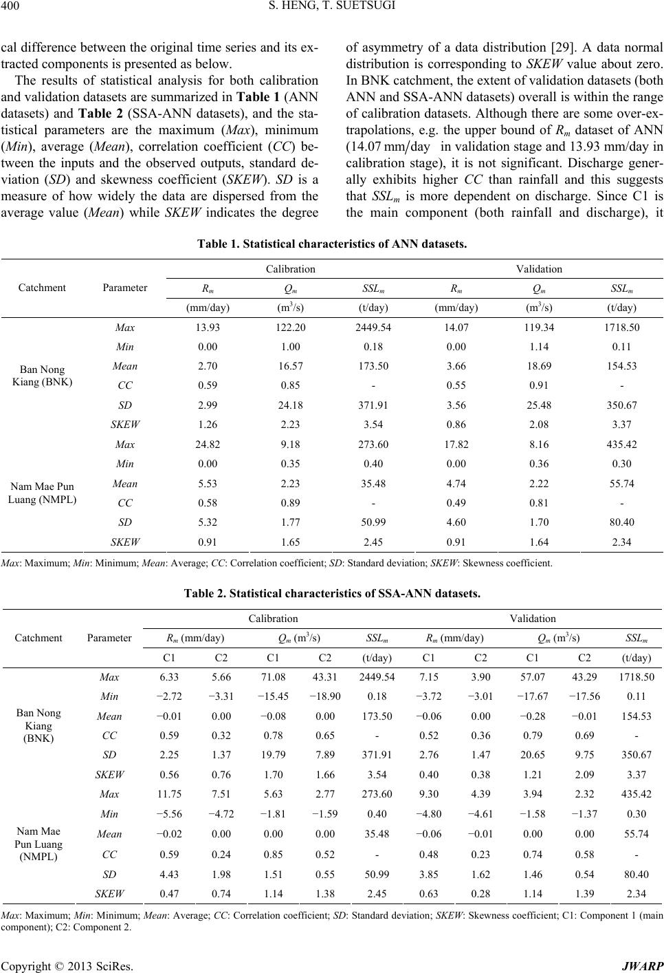

S. HENG, T. SUETSUGI 400
cal difference between the original time series and its ex-
tracted components is presented as below.
The results of statistical analysis for both calibration
and validation datasets are summarized in Table 1 (ANN
datasets) and Table 2 (SSA-ANN datasets), and the sta-
tistical parameters are the maximum (Max), minimum
(Min), average (Mean), correlation coefficient (CC) be-
tween the inputs and the observed outputs, standard de-
viation (SD) and skewness coefficient (SKEW). SD is a
measure of how widely the data are dispersed from the
average value (Mean) while SKEW indicates the degree
of asymmetry of a data distribution [29]. A data normal
distribution is corresponding to SKEW value about zero.
In BNK catchment, the extent of validation datasets (both
ANN and SSA-ANN datasets) overall is within the range
of calibration datasets. Although there are some over-ex-
trapolations, e.g. the upper bound of Rm dataset of ANN
(14.07mmday in validation stage and 13.93 mm/day in
calibration stage), it is not significant. Discharge gener-
ally exhibits higher CC than rainfall and this suggests
that SSL m is more dependent on discharge. Since C1 is
the main component (both rainfall and discharge), it
Table 1. Statistical characteristics of ANN datasets.
Calibration Validation
Rm Q
m SSLm R m Q m SSLm
Catchment Parameter
(mm/day) (m3/s) (t/day) (mm/day) (m3/s) (t/day)
Max 13.93 122.20 2449.54 14.07 119.34 1718.50
Min 0.00 1.00 0.18 0.00 1.14 0.11
Mean 2.70 16.57 173.50 3.66 18.69 154.53
CC 0.59 0.85 - 0.55 0.91 -
SD 2.99 24.18 371.91 3.56 25.48 350.67
Ban Nong
Kiang (BNK)
SKEW 1.26 2.23 3.54 0.86 2.08 3.37
Max 24.82 9.18 273.60 17.82 8.16 435.42
Min 0.00 0.35 0.40 0.00 0.36 0.30
Mean 5.53 2.23 35.48 4.74 2.22 55.74
CC 0.58 0.89 - 0.49 0.81 -
SD 5.32 1.77 50.99 4.60 1.70 80.40
Nam Mae Pun
Luang (NMPL)
SKEW 0.91 1.65 2.45 0.91 1.64 2.34
Max: Maximum; Min: Minimum; Mean: Average; CC: Correlation coefficient; SD: Standard deviation; SKEW: Skewness coefficient.
Table 2. Statistical characteristics of SSA-ANN datasets.
Calibration Validation
Rm (mm/day) Qm (m3/s) SSLm R
m (mm/day) Qm (m3/s) SSLm
Catchment Parameter
C1 C2 C1 C2 (t/day)C1 C2 C1 C2 (t/day)
Max 6.33 5.66 71.08 43.31 2449.547.15 3.90 57.07 43.29 1718.50
Min −2.72 −3.31 −15.45 −18.900.18 −3.72 −3.01 −17.67 −17.560.11
Mean −0.01 0.00 −0.08 0.00 173.50−0.06 0.00 −0.28 −0.01 154.53
CC 0.59 0.32 0.78 0.65 - 0.52 0.36 0.79 0.69 -
SD 2.25 1.37 19.79 7.89 371.912.76 1.47 20.65 9.75 350.67
Ban Nong
Kiang
(BNK)
SKEW 0.56 0.76 1.70 1.66 3.54 0.40 0.38 1.21 2.09 3.37
Max 11.75 7.51 5.63 2.77 273.609.30 4.39 3.94 2.32 435.42
Min −5.56 −4.72 −1.81 −1.59 0.40 −4.80 −4.61 −1.58 −1.37 0.30
Mean −0.02 0.00 0.00 0.00 35.48 −0.06 −0.01 0.00 0.00 55.74
CC 0.59 0.24 0.85 0.52 - 0.48 0.23 0.74 0.58 -
SD 4.43 1.98 1.51 0.55 50.99 3.85 1.62 1.46 0.54 80.40
Nam Mae
Pun Luang
(NMPL)
SKEW 0.47 0.74 1.14 1.38 2.45 0.63 0.28 1.14 1.39 2.34
Max: Maximum; Min: Minimum; Mean: Average; CC: Correlation coefficient; SD: Standard deviation; SKEW: Skewness coefficient; C1: Component 1 (main
component); C2: Component 2.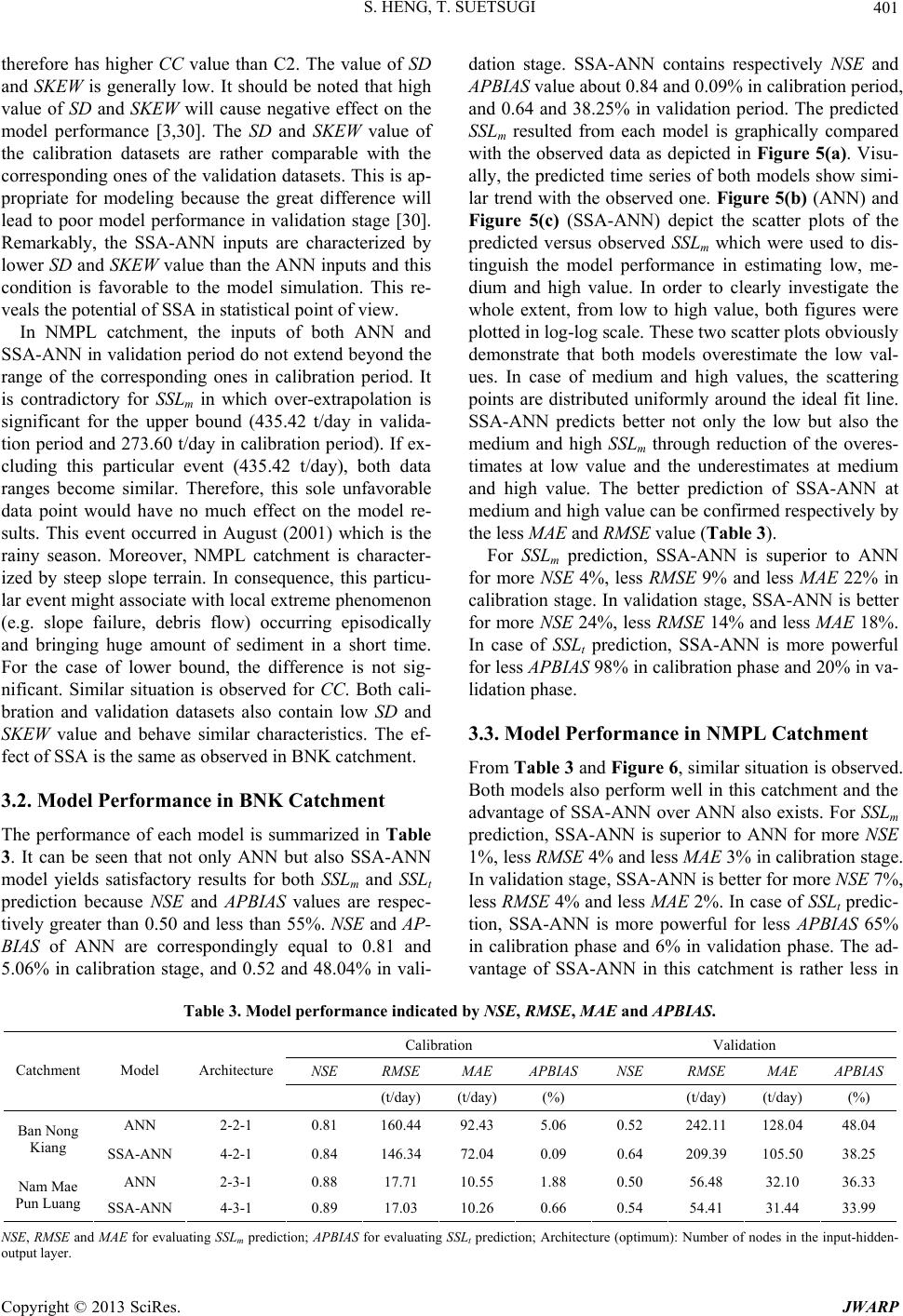

S. HENG, T. SUETSUGI 401
therefore has higher CC value than C2. The value of SD
and SKEW is generally low. It should be noted that high
value of SD and SKEW will cause negative effect on the
model performance [3,30]. The SD and SKEW value of
the calibration datasets are rather comparable with the
corresponding ones of the validation datasets. This is ap-
propriate for modeling because the great difference will
lead to poor model performance in validation stage [30].
Remarkably, the SSA-ANN inputs are characterized by
lower SD and SKEW value than the ANN inputs and this
condition is favorable to the model simulation. This re-
veals the potential of SSA in statistical point of view.
In NMPL catchment, the inputs of both ANN and
SSA-ANN in validation period do not extend beyond the
range of the corresponding ones in calibration period. It
is contradictory for SSLm in which over-extrapolation is
significant for the upper bound (435.42 t/day in valida-
tion period and 273.60 t/day in calibration period). If ex-
cluding this particular event (435.42 t/day), both data
ranges become similar. Therefore, this sole unfavorable
data point would have no much effect on the model re-
sults. This event occurred in August (2001) which is the
rainy season. Moreover, NMPL catchment is character-
ized by steep slope terrain. In consequence, this particu-
lar event might associate with local extreme phenomenon
(e.g. slope failure, debris flow) occurring episodically
and bringing huge amount of sediment in a short time.
For the case of lower bound, the difference is not sig-
nificant. Similar situation is observed for CC. Both cali-
bration and validation datasets also contain low SD and
SKEW value and behave similar characteristics. The ef-
fect of SSA is the same as observed in BNK catchment.
3.2. Model Performance in BNK Catchment
The performance of each model is summarized in Table
3. It can be seen that not only ANN but also SSA-ANN
model yields satisfactory results for both SSLm and SSLt
prediction because NSE and APBIAS values are respec-
tively greater than 0.50 and less than 55%. NSE and AP-
BIAS of ANN are correspondingly equal to 0.81 and
5.06% in calibration stage, and 0.52 and 48.04% in vali-
dation stage. SSA-ANN contains respectively NSE and
APBIAS value about 0.84 and 0.09% in calibration period,
and 0.64 and 38.25% in validation period. The predicted
SSLm resulted from each model is graphically compared
with the observed data as depicted in Figure 5(a). Visu-
ally, the predicted time series of both models show simi-
lar trend with the observed one. Figure 5(b) (ANN) and
Figure 5(c) (SSA-ANN) depict the scatter plots of the
predicted versus observed SSLm which were used to dis-
tinguish the model performance in estimating low, me-
dium and high value. In order to clearly investigate the
whole extent, from low to high value, both figures were
plotted in log-log scale. These two scatter plots obviously
demonstrate that both models overestimate the low val-
ues. In case of medium and high values, the scattering
points are distributed uniformly around the ideal fit line.
SSA-ANN predicts better not only the low but also the
medium and high SSLm through reduction of the overes-
timates at low value and the underestimates at medium
and high value. The better prediction of SSA-ANN at
medium and high value can be confirmed respectively by
the less MAE and RMSE value (Table 3).
For SS Lm prediction, SSA-ANN is superior to ANN
for more NSE 4%, less RMSE 9% and less MAE 22% in
calibration stage. In validation stage, SSA-ANN is better
for more NSE 24%, less RMSE 14% and less MAE 18%.
In case of SSLt prediction, SSA-ANN is more powerful
for less APBIAS 98% in calibration phase and 20% in va-
lidation phase.
3.3. Model Performance in NMPL Catchment
From Table 3 and Figure 6, similar situation is observed.
Both models also perform well in this catchment and the
advantage of SSA-ANN over ANN also exists. For SSLm
prediction, SSA-ANN is superior to ANN for more NSE
1%, less RMSE 4% and less MAE 3% in calibration stage.
In validation stage, SSA-ANN is better for more NSE 7%,
less RMSE 4% and less MAE 2%. In case of SSLt predic-
tion, SSA-ANN is more powerful for less APBIAS 65%
in calibration phase and 6% in validation phase. The ad-
vantage of SSA-ANN in this catchment is rather less in
Table 3. Model performance indicated by NSE, RMSE, MAE and APBIAS.
Calibration Validation
NSE RMSE MAE APBIASNSE RMSE MAE APBIAS
Catchment Model Architecture
(t/day) (t/day) (%) (t/day) (t/day) (%)
ANN 2-2-1 0.81 160.44 92.43 5.06 0.52 242.11 128.04 48.04
Ban Nong
Kiang SSA-ANN 4-2-1 0.84 146.34 72.04 0.09 0.64 209.39 105.50 38.25
ANN 2-3-1 0.88 17.71 10.55 1.88 0.50 56.48 32.10 36.33
Nam Mae
Pun Luang SSA-ANN 4-3-1 0.89 17.03 10.26 0.66 0.54 54.41 31.44 33.99
NSE, RMSE and MAE for evaluating SSLm prediction; APBIAS for evaluating SSLt prediction; Architecture (optimum): Number of nodes in the input-hidden-
output layer.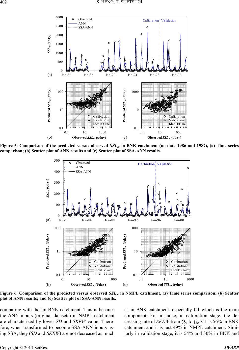

S. HENG, T. SUETSUGI 402
0
500
1000
1500
2000
2500
3000
Jan-82 Jan-86 Jan-90 Jan-94 Jan-98
SSL
m
(t/day)
Jan-02
Obser ved
ANN
SSA-ANN
0.1
10
1000
0.110 1000
Predicted SSL
m
(t/ day)
Observed SSL
m
(t/day)
Calibration
Validation
Ideal fit line
0.1
10
1000
0.1 10
Predicted SSL
m
(t/ day)
Observed SSL
m
1000
(t/ day)
Ca libra tio n
Validation
Ideal fit line
Calibration Valida
(b)
(a)
(c)
tion
Figure 5. Comparison of the predicted versus observed SSLm in BNK catchment (no data 1986 and 1987), (a) Time series
comparison; (b) Scatter plot of ANN results and (c) Scatter plot of SSA-ANN results.
0
100
200
300
400
500
Jan-80 Jan-84 Jan-88 Jan-92 Jan-96
SSL
m
(t/ day)
Jan-00
Observed
ANN
SSA-ANN
0.1
10
1000
0.110 1000
Predic ted SSL
m
(t/day)
Observed SSL
m
(t/day)
Ca libra tion
Va lidation
Ideal fit line
0.1
10
1000
0.1 10
Predic ted SSL
m
(t/day)
Observ ed SS
1000
L
m
(t/day)
Calibra tion
Validation
Calibration Validat
(b)
(a)
(c)
Ideal fit line
ion
Figure 6. Comparison of the predicted versus observed SSLm in NMPL catchment, (a) Time series comparison; (b) Scatter
plot of ANN results; and (c) Scatter plot of SSA-ANN results.
comparing with that in BNK catchment. This is because
the ANN inputs (original datasets) in NMPL catchment
are characterized by lower SD and SKEW value. There-
fore, when transformed to become SSA-ANN inputs us-
ing SSA, they (SD and SKEW) are not decreased as much
as in BNK catchment, especially C1 which is the main
component. For instance, in calibration stage, the de-
creasing rate of SKEW from Qm to Qm-C1 is 56% in BNK
catchment and it is just 49% in NMPL catchment. Simi-
larly in validation stage, it is 54% and 30% in BNK and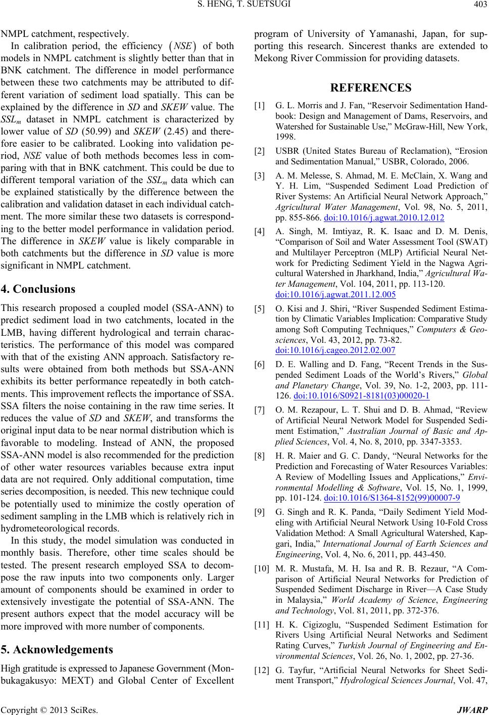

S. HENG, T. SUETSUGI 403
NMPL catchment, respectively.
In calibration period, the efficiency of both
models in NMPL catchment is slightly better than that in
BNK catchment. The difference in model performance
between these two catchments may be attributed to dif-
ferent variation of sediment load spatially. This can be
explained by the difference in SD and SKEW value. The
SSLm dataset in NMPL catchment is characterized by
lower value of SD (50.99) and SKEW (2.45) and there-
fore easier to be calibrated. Looking into validation pe-
riod, NSE value of both methods becomes less in com-
paring with that in BNK catchment. This could be due to
different temporal variation of the SSLm data which can
be explained statistically by the difference between the
calibration and validation dataset in each individual catch-
ment. The more similar these two datasets is correspond-
ing to the better model performance in validation period.
The difference in SKEW value is likely comparable in
both catchments but the difference in SD value is more
significant in NMPL catchment.

NSE
4. Conclusions
This research proposed a coupled model (SSA-ANN) to
predict sediment load in two catchments, located in the
LMB, having different hydrological and terrain charac-
teristics. The performance of this model was compared
with that of the existing ANN approach. Satisfactory re-
sults were obtained from both methods but SSA-ANN
exhibits its better performance repeatedly in both catch-
ments. This improvement reflects the importance of SSA.
SSA filters the noise containing in the raw time series. It
reduces the value of SD and SKEW, and transforms the
original input data to be near normal distribution which is
favorable to modeling. Instead of ANN, the proposed
SSA-ANN model is also recommended for the prediction
of other water resources variables because extra input
data are not required. Only additional computation, time
series decomposition, is needed. This new technique could
be potentially used to minimize the costly operation of
sediment sampling in the LMB which is relatively rich in
hydrometeorological records.
In this study, the model simulation was conducted in
monthly basis. Therefore, other time scales should be
tested. The present research employed SSA to decom-
pose the raw inputs into two components only. Larger
amount of components should be examined in order to
extensively investigate the potential of SSA-ANN. The
present authors expect that the model accuracy will be
more improved with more number of components.
5. Acknowledgements
High gratitude is expressed to Japanese Government (Mon-
bukagakusyo: MEXT) and Global Center of Excellent
program of University of Yamanashi, Japan, for sup-
porting this research. Sincerest thanks are extended to
Mekong River Commission for providing datasets.
REFERENCES
[1] G. L. Morris and J. Fan, “Reservoir Sedimentation Hand-
book: Design and Management of Dams, Reservoirs, and
Watershed for Sustainable Use,” McGraw-Hill, New York,
1998.
[2] USBR (United States Bureau of Reclamation), “Erosion
and Sedimentation Manual,” USBR, Colorado, 2006.
[3] A. M. Melesse, S. Ahmad, M. E. McClain, X. Wang and
Y. H. Lim, “Suspended Sediment Load Prediction of
River Systems: An Artificial Neural Network Approach,”
Agricultural Water Management, Vol. 98, No. 5, 2011,
pp. 855-866. doi:10.1016/j.agwat.2010.12.012
[4] A. Singh, M. Imtiyaz, R. K. Isaac and D. M. Denis,
“Comparison of Soil and Water Assessment Tool (SWAT)
and Multilayer Perceptron (MLP) Artificial Neural Net-
work for Predicting Sediment Yield in the Nagwa Agri-
cultural Watershed in Jharkhand, India,” Agricultural Wa-
ter Management, Vol. 104, 2011, pp. 113-120.
doi:10.1016/j.agwat.2011.12.005
[5] O. Kisi and J. Shiri, “River Suspended Sediment Estima-
tion by Climatic Variables Implication: Comparative Study
among Soft Computing Techniques,” Computers & Geo-
sciences, Vol. 43, 2012, pp. 73-82.
doi:10.1016/j.cageo.2012.02.007
[6] D. E. Walling and D. Fang, “Recent Trends in the Sus-
pended Sediment Loads of the World’s Rivers,” Global
and Planetary Change, Vol. 39, No. 1-2, 2003, pp. 111-
126. doi:10.1016/S0921-8181(03)00020-1
[7] O. M. Rezapour, L. T. Shui and D. B. Ahmad, “Review
of Artificial Neural Network Model for Suspended Sedi-
ment Estimation,” Australian Journal of Basic and Ap-
plied Sciences, Vol. 4, No. 8, 2010, pp. 3347-3353.
[8] H. R. Maier and G. C. Dandy, “Neural Networks for the
Prediction and Forecasting of Water Resources Variables:
A Review of Modelling Issues and Applications,” Envi-
ronmental Modelling & Software, Vol. 15, No. 1, 1999,
pp. 101-124. doi:10.1016/S1364-8152(99)00007-9
[9] G. Singh and R. K. Panda, “Daily Sediment Yield Mod-
eling with Artificial Neural Network Using 10-Fold Cross
Validation Method: A Small Agricultural Watershed, Kap-
gari, India,” International Journal of Earth Sciences and
Engineering, Vol. 4, No. 6, 2011, pp. 443-450.
[10] M. R. Mustafa, M. H. Isa and R. B. Rezaur, “A Com-
parison of Artificial Neural Networks for Prediction of
Suspended Sediment Discharge in River—A Case Study
in Malaysia,” World Academy of Science, Engineering
and Technology, Vol. 81, 2011, pp. 372-376.
[11] H. K. Cigizoglu, “Suspended Sediment Estimation for
Rivers Using Artificial Neural Networks and Sediment
Rating Curves,” Turkish Journal of Engineering and En-
vironmental Sciences, Vol. 26, No. 1, 2002, pp. 27-36.
[12] G. Tayfur, “Artificial Neural Networks for Sheet Sedi-
ment Transport,” Hydrological Sciences Journal, Vol. 47,

S. HENG, T. SUETSUGI 404
No. 6, 2002, pp. 879-892.
doi:10.1080/02626660209492997
[13] O. Kisi, “Development of Streamflow-Suspended Sedi-
ments Rating Curve Using a Range Dependent Neural
Network,” International Journal of Science and Tech-
nology, Vol. 2, No. 1, 2007, pp. 49-61.
[14] C. Sivapragasam, S.-Y. Liong and M. F. K. Pasha, “Rain-
fall and Runoff Forecasting with SSA-SVM Approach,”
Journal of Hydroinformatics, Vol. 3, No. 3, 2001, pp. 141-
152.
[15] N. Golyandina, V. Nekrutkin and A. A. Zhigljavsky, “Ana-
lysis of Time Series Structure: SSA and Related Tech-
niques,” Chapman and Hall/CRC, Boca Raton, 2001.
doi:10.1201/9781420035841
[16] GistaT Group, “Time Series Analysis and Forecasting,”
2010. http://www.gistatgroup.com/cat/
[17] R. T. Hanson, M. W. Newhouse and M. D. Dettinger, “A
Methodology to Assess Relations between Climatic Va-
riability and Variations in Hydrologic Time Series in the
Southwestern United States,” Journal of Hydrology, Vol.
287, No. 1-4, 2004, pp. 252-269.
doi:10.1016/j.jhydrol.2003.10.006
[18] C. A. F. Marques, J. A. Ferreira, A. Rocha, J. M. Castan-
heira, P. Melo-Goncalves, N. Vaz and J. M. Dias, “Sin-
gular Spectrum Analysis and Forecasting of Hydrological
Time Series,” Physics and Chemistry of the Earth, Vol.
31, No. 18, 2006, pp. 1172-1179.
doi:10.1016/j.pce.2006.02.061
[19] H. J. Fuchs, “Data Availability for Studies on Effects of
Land-Cover Changes on Water Yield, Sediment and Nu-
trient Load at Catchments of the Lower Mekong Basin,”
MRC-GTZ Cooperation Programme, Göttingen, 2004.
[20] H. Memarian and S. K. Balasundram, “Comparison be-
tween Multi-Layer Perceptron and Radial Basis Function
Networks for Sediment Load Estimation in a Tropical
Watershed,” Journal of Water Resource and Protection,
Vol. 4, No. 10, 2012, pp. 870-876.
doi:10.4236/jwarp.2012.410102
[21] S. Heng and T. Suetsugi, “Using Artificial Neural Net-
work to Estimate Sediment Load in Ungauged Catch-
ments of the Tonle Sap River Basin, Cambodia,” Journal
of Water Resource and Protection, Vol. 5, No. 2, 2013,
pp. 111-123. doi:10.4236/jwarp.2013.52013
[22] Y. Tramblay, A. St-Hilaire and T. B. M. J. Ouarda, “Fre-
quency Analysis of Maximum Annual Suspended Sedi-
ment Concentrations in North America,” Hydrological
Sciences Journal, Vol. 53, No. 1, 2008, pp. 236-252.
doi:10.1623/hysj.53.1.236
[23] P. Gao and M. Josefson, “Event-Based Suspended Sedi-
ment Dynamics in a Central New York Watershed,” Geo-
morphology, Vol. 139-140, 2011, pp. 425-437.
doi:10.1016/j.geomorph.2011.11.007
[24] S. Heng and T. Suetsugi, “Estimating Quantiles of An-
nual Maximum Suspended Sediment Load in the Tribu-
taries of the Lower Mekong River,” Journal of Water and
Climate Change, Vol. 4, No. 1, 2013, pp. 63-76.
doi:10.2166/wcc.2013.023
[25] O. Kisi, I. Yuksel and E. Dogan, “Modelling Daily Sus-
pended Sediment of Rivers in Turkey Using Several
Data-Driven Techniques,” Hydrological Sciences Journal,
Vol. 53, No. 6, 2008, pp. 1270-1285.
doi:10.1623/hysj.53.6.1270
[26] O. Kisi, “Multi-Layer Perceptrons with Levenberg-Mar-
quardt Training Algorithm for Suspended Sediment Con-
centration Prediction and Estimation,” Hydrological Sci-
ences Journal, Vol. 49, No. 6, 2004, pp. 1025-1040.
doi:10.1623/hysj.49.6.1025.55720
[27] J. E. Nash and J. V. Sutcliffe, “River Flow Forecasting
through Conceptual Models Part I-A Discussion of Prin-
ciples,” Journal of Hydrology, Vol. 10, No. 3, 1970, pp.
282-290. doi:10.1016/0022-1694(70)90255-6
[28] D. N. Moriasi, J. G. Arnold, M. W. V. Liew, R. L. Bing-
ner, R. D. Harmel and T. L. Veith, “Model Evaluation
Guidelines for Systematic Quantification of Accuracy in
Watershed Simulations,” Transactions of the American
Society of Agriculture and Biological Engineers, Vol. 50,
No. 3, 2007, pp. 885-900.
[29] M. Shahin, H. J. L. Van Oorschot and S. J. De Lange,
“Statistical Analysis in Water Resources Engineering,” A.
A. Balkema, Rotterdam, 1993.
[30] T. Rajaee, “Wavelet and ANN Combination Model for
Prediction of Daily Suspended Sediment Load in Rivers,”
Science of the Total Environment, Vol. 409, No. 15, 2010,
pp. 2917-2928. doi:10.1016/j.scitotenv.2010.11.028