Applied Mathematics
Vol.3 No.10A(2012), Article ID:24101,9 pages DOI:10.4236/am.2012.330206
Non-Frobenius Spectrum-Transformation Method
1Department of Management, Concern Morinformsystem-Agat, Joint Stock Company, Moscow, Russia
2Department of Management, Military-Industrial Commission of the Russian Federation, Moscow, Russia
3Department of Automatics, Institute of Shipbuilding and Marine Arctic Equipment, Severodvinsk, Russia
Email: asiskhakov@mail.ru, vyapospelov@mail.ru, skovpensm@mail.ru
Received July 10, 2012; revised August 10, 2012; accepted August 17, 2012
Keywords: Matrix Spectrum; Modal Control; Spectrum Transformation; Frobenius Matrix; Linear Spectral Transformation; Non-Frobenius Transformation
ABSTRACT
A method allowing a desirable matrix spectrum to be constructed as an alternative to the method using matrix transformation to the Frobenius form is stated. It can be applied to implement control algorithms for technical systems without executing the variables transformation procedures that are needed for deriving a Frobenius matrix. The method can be used for simulation of systems with different spectrums for choosing an alternative that satisfies to the distinct demands.
1. Introduction
A number of mathematical problems deal with changes of a matrix spectrum [1,2]. It can be changed by various methods, for example, in computing problems, a multiplication to other matrix is used. In control problems, to change a spectrum, a matrix is added with some other matrix derivated by a feedback, which forms a linear function of variables. This approach is known as modal control [3,4] or spectrum control [5].
To solve the above problems and to obtain a matrix with required eigenvalues a matrix is reduced to the Frobenius form. This transformation called here Frobenius, has a clear foundation and it is widely applied as theoretical tool. However, an attempt to use this approach for practical control problems with implementation of control algorithms by concrete technical devices has shown that such method is of limited application.
The matter is that in technical systems so-called physical variables are used. These latter characterize energy storage units, in particular, a velocity of a moving mass, a solenoid coil current, a voltage of a capacitor and similar. The values of physical variables are gained from sensors. In order to obtain a Frobenius matrix it is necessary to transform physical variables of feedback loop. In this case the transformation is double, because just a combination of physical variables must goes to the input. To execute such transformations it is required an additional either hardware expenditures or time delays in program implementation.
In this paper, the method of obtaining a desirable spectrum without resort to a Frobenius matrix is stated. It also can be used for calculating the feedback coefficients of a control system for the purpose to derive a desirable spectrum. It enables one to solve the control problems by simulating a system behavior with different spectrums for searching a comprehensible alternative. Among them the most demanded for practical applications it is possible to consider the spectrum correction problem, when it is required to determine parameters of a feedback for altering a part of a spectrum.
2. Description of the Method
2.1. Informative Side
The Frobenius transformation is based on the relationship between eigenvalues and coefficients of a characteristic polynomial of a matrix in which a row is formed from these coefficients. The additive action of the feedback confirming an operation of summing the elements of a row with the elements of the feedback changes a row and a spectrum as well. The feedback elements are computed evidently as the differences between elements of a Frobenius matrix row and the coefficients of a polynomial of a matrix having a given spectrum.
The presented method is based on a relation between elements and eigenvalues of a matrix. For identity of system with the numbers that do not belong to a matrix spectrum, some of the elements are replaced by the unknowns. Solving a system of equations for unknowns one gives a desired spectrum of a matrix.
2.2. Purpose Statement
Let  be a given real k by k matrix, where i, j
 . A matrix spectrum σ(А) contains a real set
 ,
,  , where
  is the given set of l real numbers, and k ≥ l ≥ 1.
A matrix having a spectrum that in full or in part coincides with Λ, obtained by replacing some of its elements we denote by Аx. For two alternatives of the spectrum setting we have:
1) l < k is a part of a spectrum
2) l = k is whole spectrum.
The goal is to find the replaced elements.
2.3. The Non-Frobenius Transformation of a Matrix Spectrum
For the matrix А we write the equalities
 (1)
(1)
where bi is the sum of all main minors of i order, and ci are the coefficients of a characteristic polynomial.
Definition 1. Changeover the element аi,j in matrix A by the unknown elements xi,j is called the replacement, xi,j is the replaced element, the matrix having l replaced elements is called the replaced matrix and it is denoted by Аx.
Definition 2. The non-Frobenius transformation of a matrix spectrum, further the spectral transformation, is called the substitution of any its l elements by the result of a solution of the system (1) for the replaced matrix
 (2)
(2)
concerning replaced elements, where gi has the same sense as coefficient bi, the coefficient di is derivated from l numbers of the set Λ and from (k − l) unknowns of a spectrum.
For l < k the equalities (2) become a system of equations for l replaced elements and (k − l) unknowns of a spectrum. A solution of this system enables one to specify them in the form of a function of the remaining elements of the matrix A and the elements of the set Λ.
Definition 3. The spectral transformation for l < k is called the incomplete one.
An example of the incomplete spectral transformation for l < k is resulted in Appendix A. Further the case with l = k is observed as more demanded for practical applications. In this case the spectral transformation enables one to change certain eigenvalues, while the remaining part of a spectrum is unchanged, otherwise, such transformation control over a spectrum.
Let’s collect the elements xi,j into the vector x. Generally, the equalities (2) represent a system of equations for the vector x
 (3)
(3)
where F is a nonlinear vector function of k size. The type of the system (3) depends on allocation of the elements of vector x in the replaced matrix. If they allocate in different rows and columns, as it is shown in an example for replaced matrix
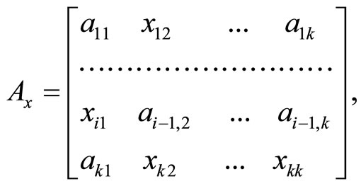 (4)
(4)
the system is reduced to a solution of the equation of a degree from 2-nd to k-th, thus a degree of the equation is equal to a maximum number of the replaced elements in the addends of the last row of the system (3).
Definition 4. The Equation (3) is called the system of spectral transformation of i-th order, where i is a maximum number of replaced elements in the addends of the last row.
Definition 5. The system of spectral transformation of the first order is called the linear, and the transformation is called the linear spectral transformation (LST).
Definition 6. The system of spectral transformation above the first order is called the nonlinear, and transformation is called nonlinear spectral transformation (NST).
Theorem. If solution of the system (3) exists than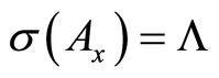 .
.
Proof. With substitution of solution of the Equation (3) into the matrix Аx the coefficients of its characteristic polynomial become equal to values of combinations of numbers of the given set Λ spotted by a right side of the system (2), which left side is identical. This completes the proof.
Further we consider that replaced elements make a row or column in replaced matrix. The LST is illustrated by numerical examples in Appendices A, B, and C.
2.4. The Row LST
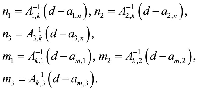
For replacing row i of the matrix A the replaced vector х is denoted by ni. The replaced matrix takes the form
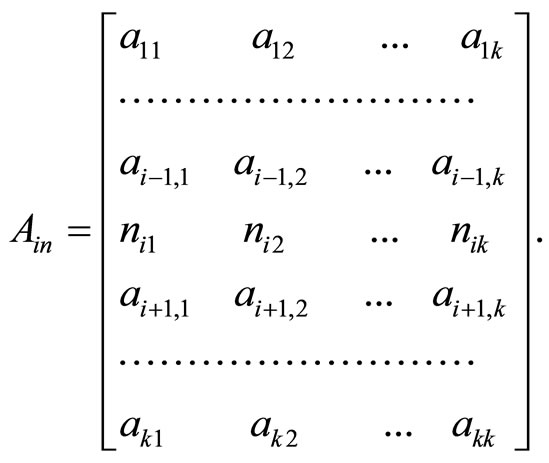 (5)
(5)
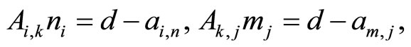
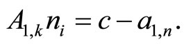
The equalities (2) for the matrix (5) in view of linearity of minors by each row vector of the matrix [6] become the LST system
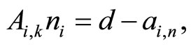 (6)
(6)
where Аi,k is a matrix,  , and аi,n is a vector.
Definition 7. The matrix Аi,k is called the LST matrix by the row i, and the condition
 (7)
(7)
is called the condition of existence of the LST matrix A by the row i.
If the condition (7) is satisfied than , i.e. the replaced matrix (5) with the solution of system (6)
 (8)
(8)
acquires a spectrum that is equal to the given set Λ. The fulfillment of (7) for  enables one to find k vectors of ni.
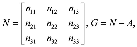
Definition 8. The matrix N involving the all rows  of (8) is called the summary matrix of rows of the LST, the matrix G = N − A is called the summary matrix of the complements of rows of the LST.
Spectrums of all matrixes derivated by replacement of an arbitrary row of the matrix A by the row of the matrix N, and also by addition of an arbitrary row of the matrix A with row having the same number of the matrix G are equal.
2.5. The Column LST
Let the elements of the vector x replace the column number j in the matrix A. This vector is denoted by mj. The replaced matrix has the form
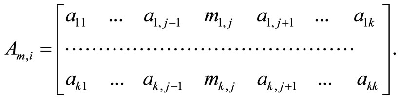 (9)
(9)
For the matrix (9) we construct the LST system
 (10)
(10)
where Аk,j is a matrix, and аm,j is a vector.
Definition 9. The matrix Аk,j is called the LST matrix by the column j, and the condition
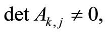 (11)
(11)
is called the condition of existence of the LST matrix A by the column j.
If the condition (11) is satisfied than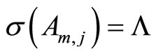 , i.e. the replaced matrix (9) with the solution of system (10)
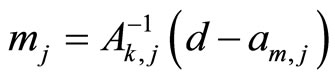 (12)
(12)
acquires a spectrum that is equal to the given set Λ. The fulfillment of (11) for  enables one to find k vectors of mj.
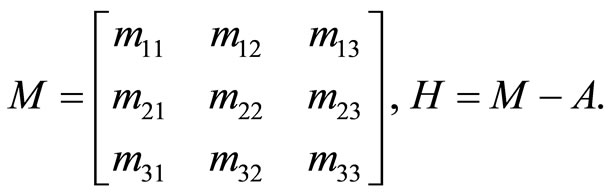
Definition 10. The matrix M involving the all columns  of (12) is called the summary matrix of columns of the LST, the matrix H = M − A is called the summary matrix of the complements of columns of the LST.
Spectrums of all matrixes derivated by replacement of an arbitrary column of the matrix A by a column with the same number of the matrix M, and also by addition of arbitrary column of the matrix A by the column with the same number of the matrix Н are equal.
2.6. Remarks
In spite of formal equivalence of row and column alternatives of the LST, their practical significance is not equal. The matter is that control systems have the single input into which the linear combination of all variables arrives that corresponds to additive action of row vector. Therefore the row alternative of the LST has a greater potential for applications in solutions of control problems.
3. Conclusion
In this paper, we proposed a new spectrum-transformation method, which enables a desirable matrix spectrum to be obtained without recourse to deriving a Frobenius matrix. Because of this the method was called the nonFrobenius transformation. The linear spectral transformation was described in detail and illustrated by the examples of spectrum transformation for matrices of the 2nd, 3rd, and 4th order. Finally, in Appendix D, we show how the LST can be used for solving a modal control problem in terms of changing matrix eigenvalues for system with unique control input.
REFERENCES
- R. Gabasov and F. M. Kirillova, “Mathematical Theory of Optimal Control. Results of Since and Engineering,” Mathematical Analysis, Vol. 16, 1979, pp. 55-97.
- G. G. Islamov, “On the Control of a Dynamical System Spectrum,” Differential Equations, Vol. 23, No. 8, 1987, pp. 1299-1302.
- N. T. Kuzovkov, “Modal Control and Observe Devices,” Mashinostroenie, Moscow, 1976.
- A. A. Krasovsky, “Control Theory Reference Book,” Nauka, Moscow, 1987.
- G. A. Leonov and M. M. Shumafov, “The Methods for Linear Controlled System Stabilization,” St.-Petersburg University Publisher, St.-Petersburg, 2005.
- V. V. Voevodin and Y. A. Kuznetsov, “Matrices and Calculations,” Nauka, Moscow, 1984.
- R. Isermann, “Digital Control Systems,” Springer-Verlag, New York, 1996
Appendix A
Case k = 2. Let’s set up the system
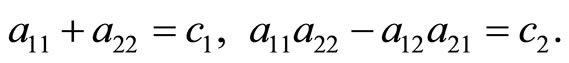 (13)
(13)
We illustrate incomplete LST for l = 1. Denoting the unknown eigenvalue by ω11, from (13) we obtain the system

We rewrite this system in the normal form
 (14)
(14)
For λ ¹ а22, the solution of (14) is given by
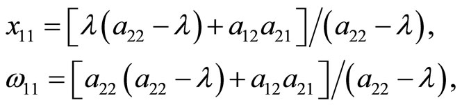 (15)
(15)
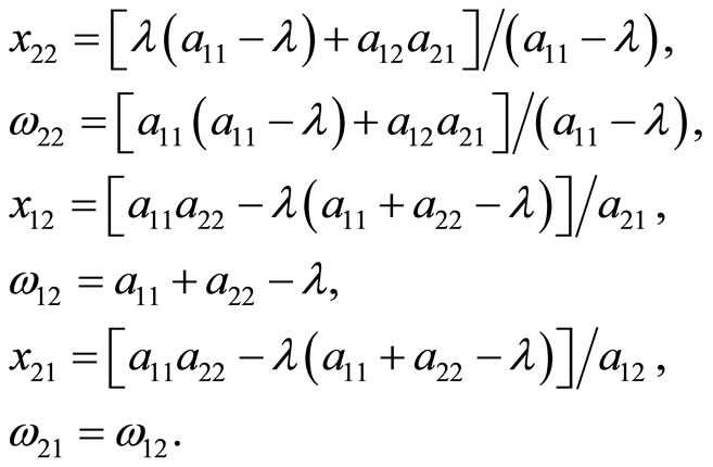
By replacing other elements, we get the solutions in a similar way:
For а11 = 3, а12 = 4, а21 = 7, а22 = 6, Σ = {–1, 10}, and λ = 2, from (15), we obtain:
 (16)
(16)
So, the required eigenvalue for incomplete LST depends on choosing the replaced element.
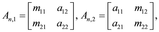
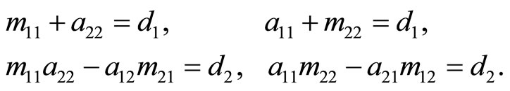
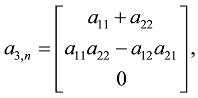
Now we explain how to determine whole spectrum. In row LST for the replaced matrices (5)
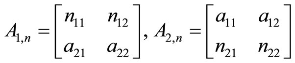 (17)
(17)
the systems (2) are given by
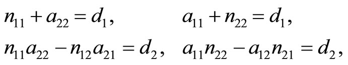 (18)
(18)
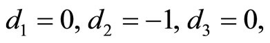
where d1 = λ1 + λ2, d2 = λ1λ2.
The systems (18) expressed in the form (6) are
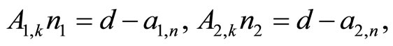 (19)
(19)
where 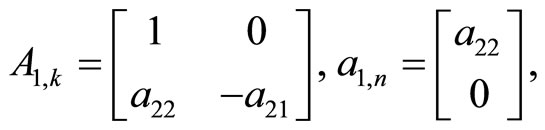
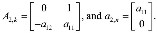
If the condition (7) −а21 ¹ 0 and а12 ¹ 0 is satisfied for each system, then these systems have the solutions
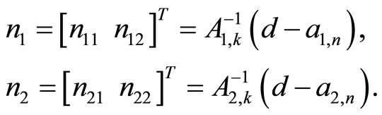 (20)
(20)
For replaced matrices (17) whose solutions are (20) the following conditions satisfy
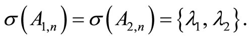 (21)
(21)
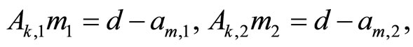
Iterating the LST for the matrices with replaced columns
 (22)
(22)
we write the systems (2) as
 (23)
(23)
In the form (10) the systems (23) are
 (24)
(24)
where 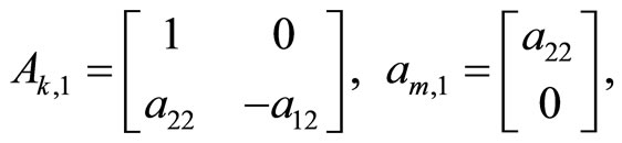
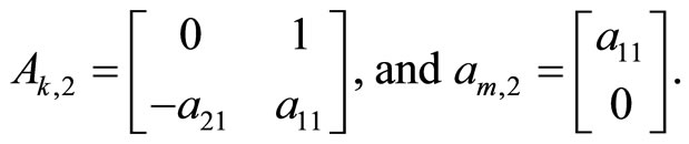
Under conditions а21 ¹ 0 and а12 ¹ 0 the systems (24) have the solutions
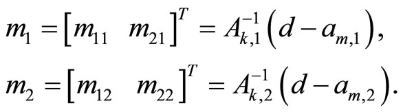 (25)
(25)
With solutions (25) the replaced matrices (22) gain the required spectrum
 (26)
(26)
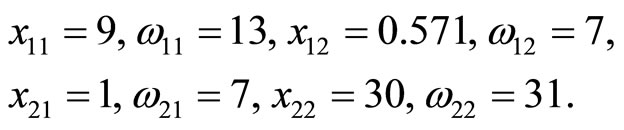
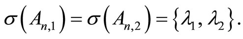
Using the numerical data from example, we generate a spectrum that is different from Σ = {−1, 10} by the number λ2 = 1. We calculate
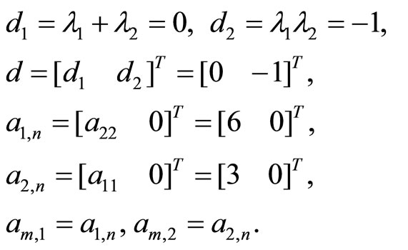
Using the expressions (20) and (25), we find the replacement vectors

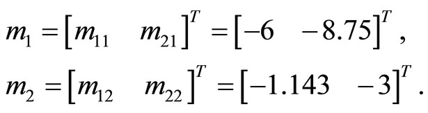
The replacement matrices (17) and (22) gain the following spectrum
that is different from spectrum of the matrix А by a single number.
Appendix B
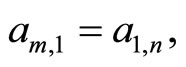
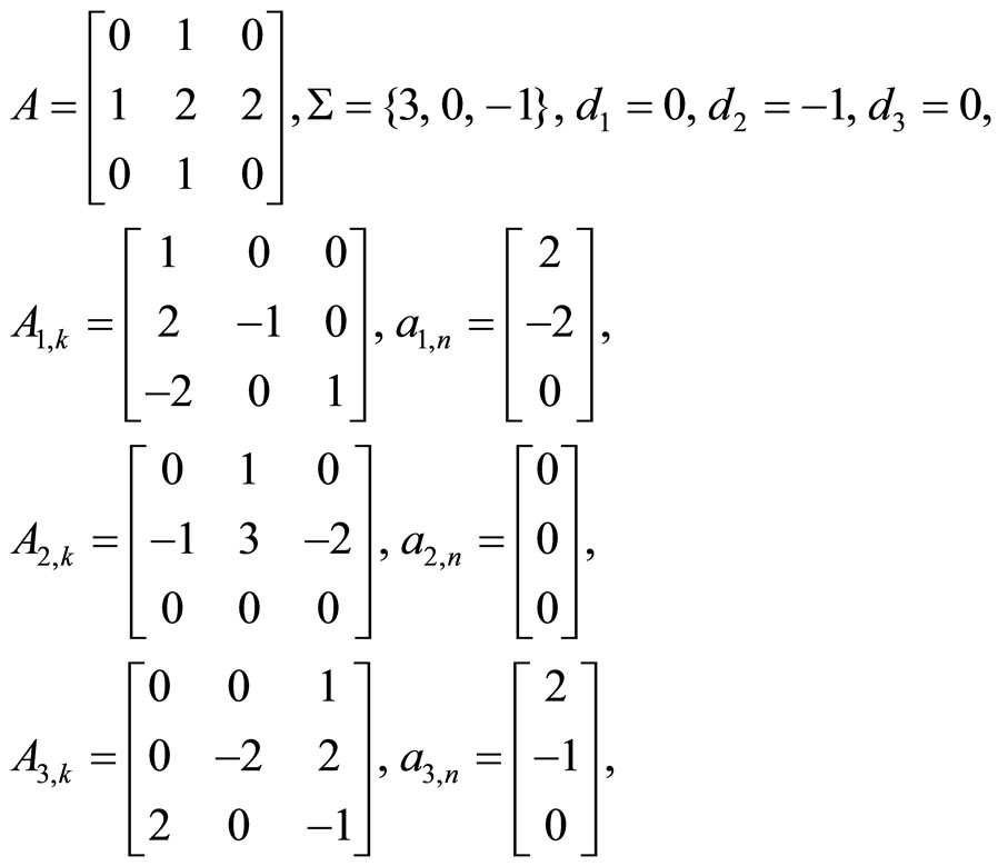
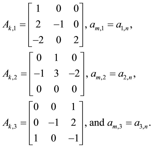
Case k = 3. From the equalities (1)
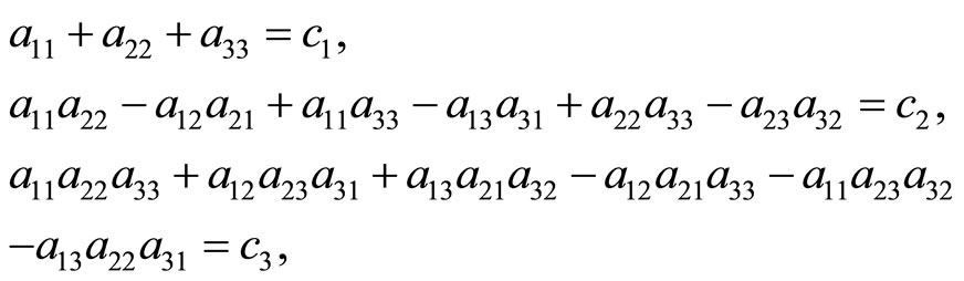
we set up the LST systems (6) and (10)
 (27)
(27)
where 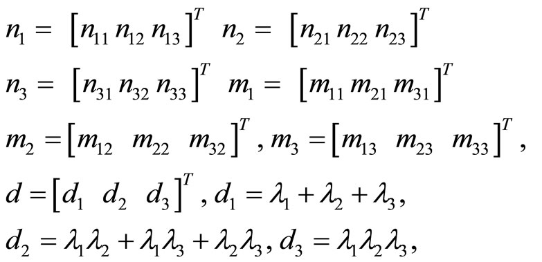
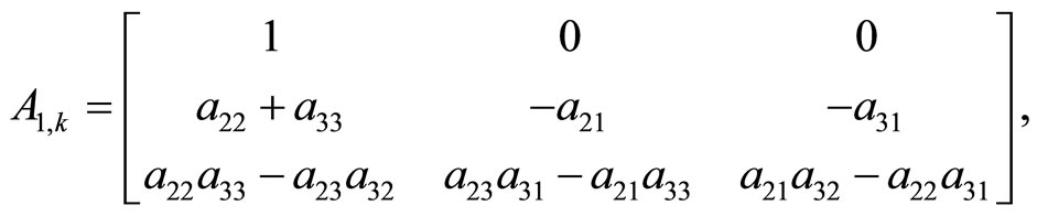
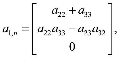


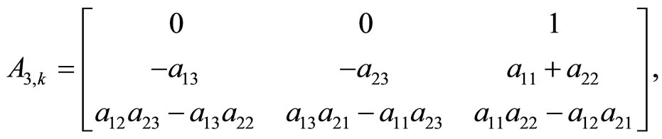
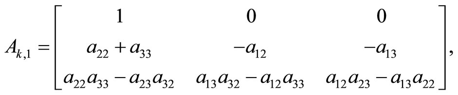
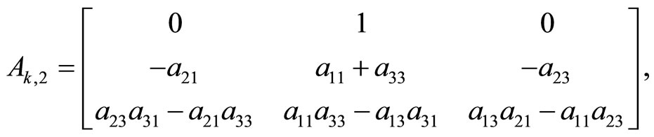


and .
.
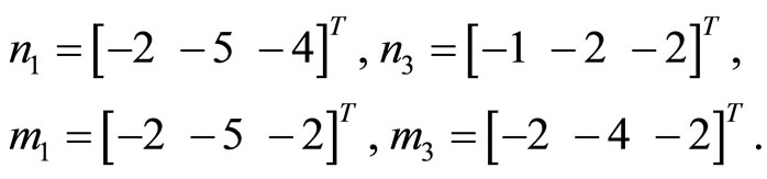
If both (7) and (11) conditions satisfy for all i and j, then the solutions of the systems (7) are
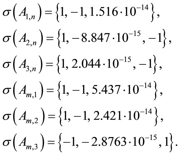
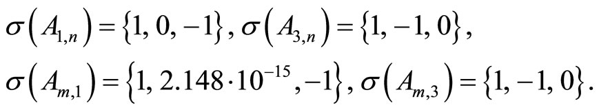
After calculating the eigenvalues of the replaced matrices
 (28)
(28)
one obtains the required set Λ:

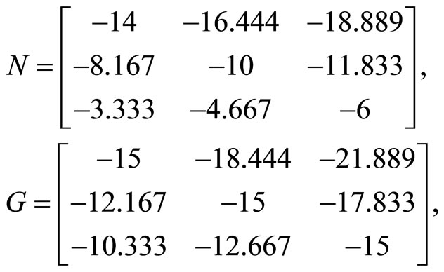
We write the summary matrices of rows and the complements of rows
 (29)
(29)
and also the summary matrices of columns and the complements of columns
 (30)
(30)
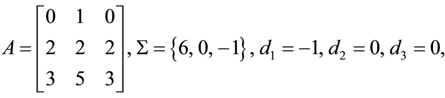
Let’s observe matrices for which LST by different rows and columns exists, Λ = {1, 0, −1}.
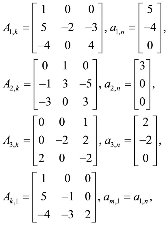
1) LST exists by all rows and columns. For the matrix
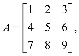
from (27), we find
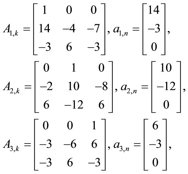
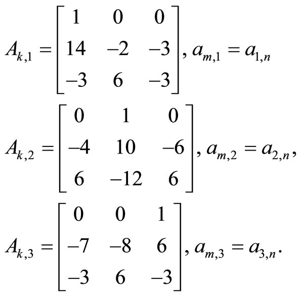 (31)
(31)
The matrices (31) are nonsingular; therefore all of systems (27) have the solutions
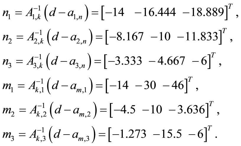
Calculating the eigenvalues of the replaced matrices one gives the required set:
The summary matrices of rows and the complements of rows (29) are
and the summary matrices of columns and the complements of columns (30) are

2) LST exists by certain rows and columns.
2.1) LST by three columns and two rows.
For the matrix
 (32)
(32)
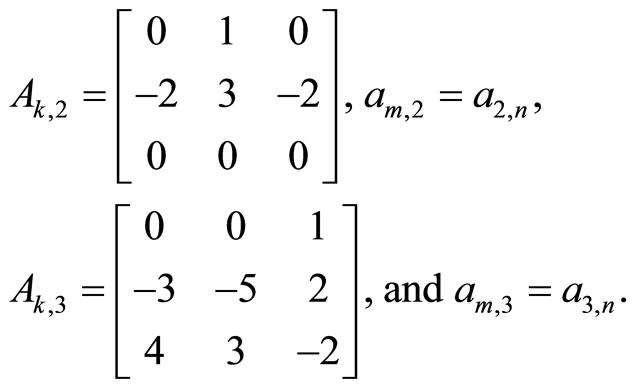
The matrix Аk,2 is singular. The solutions of the systems (27) are
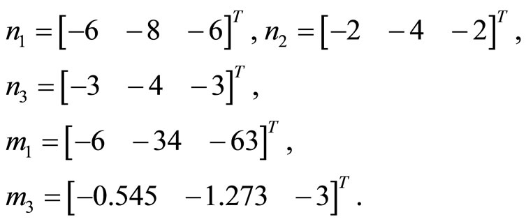
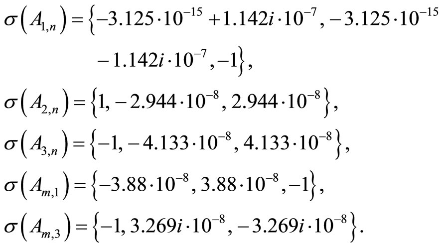
Calculating the eigenvalues of the replaced matrices one gives the required set:
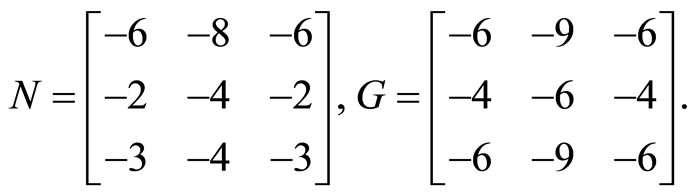
The summary matrices of rows and the complements of rows (29) are
2.2) LST by two columns and two rows.
For the matrix
The matrices А2,k and Аk,2 are singular. The solutions of the systems (27) are
The eigenvalues of the replaced matrices have the required set:
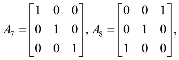
2.3) We cite the matrices (without calculations), which suppose
a) two LST:
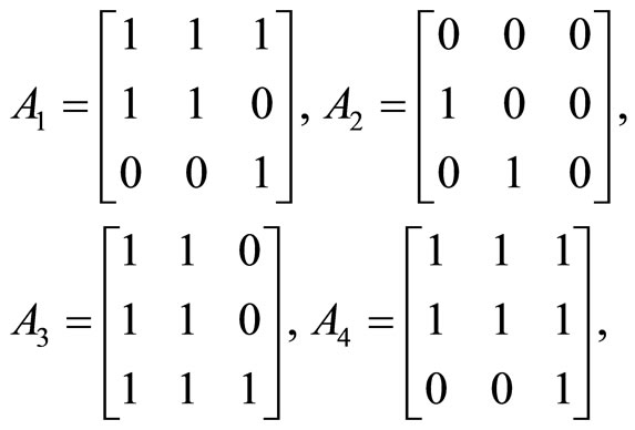
А1 for row 3 and column 2, А2 for row 1 and column 3, А3 for rows 1 and 2, and А4 for columns 1 and 2.
b) single LST:
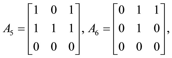
А5 for row 3, and А6 for column 1.
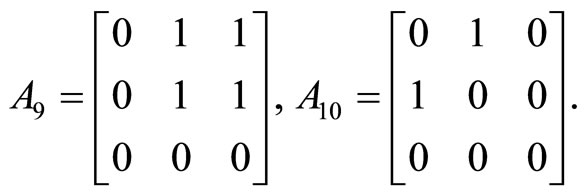
c) the following matrices do not have the LST:
Appendix C
Case k = 4. Passing over the equalities (1), we write the LST system (6) by first row at once
 (33)
(33)
where 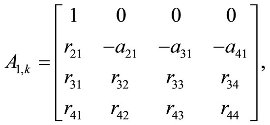
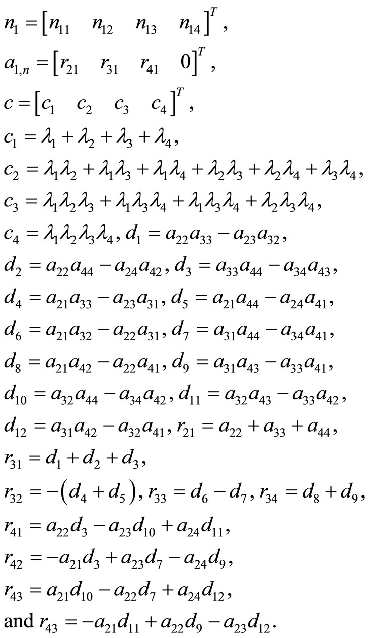
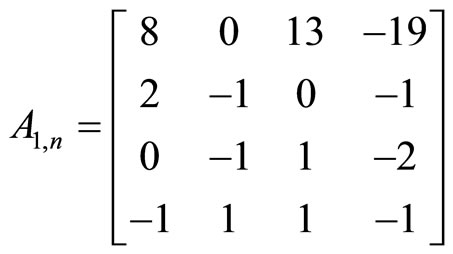
For the replaced matrix
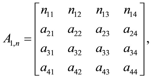 (34)
(34)
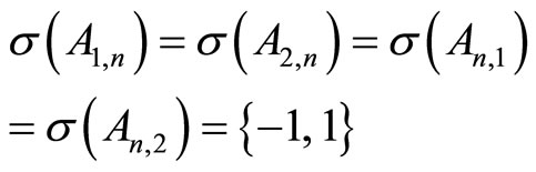
the condition σ(А1,n) = Λ satisfies.
We consider the matrix
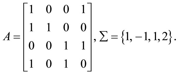
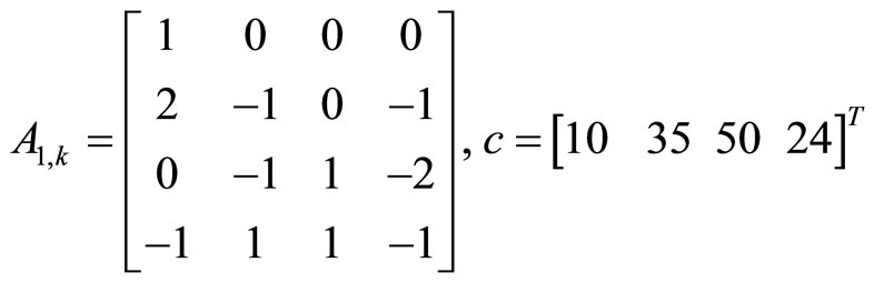
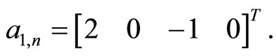
We set up the set Λ = {1, 2, 3, 4} with two numbers from Σ. Omitting the intermediate calculations, we find the elements of matrices and vectors of the system (33)
With replacement vector 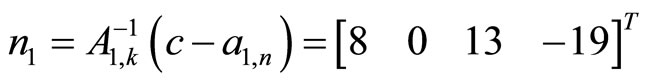 , the matrix (34)
 (35)
(35)
gains a spectrum with the required set 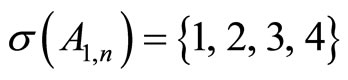 .
.
All calculations were yielded in Mathcad.
Appendix D
LST Application to the Modal Control Problem
Here, we compare the stated method to the known alternative of modal control. First of all, we recall that in accordance with up-to-date concepts of modal control, change the matrix eigenvalues independently of each other can be implemented only by separate action on the control input associated with a given eigenvalue. Thus, to implement a modal control, a system should have the number of inputs that is equal to the system order. This demand, as it is cited in a number of sources, for example, in [7], is seldom fulfilled, that is a significant constraint of the up-to-date method of modal control. The vast majority of multivariable control systems have a unique control input.
The stated transformation method allows eigenvalues to be changed independently by action to a unique input. It is possible to call this alternative method as a one-input modal control.
To compare these approaches, the simplified block diagram taken from [7] is shown in Figure 1. The functions of the blocks are clear from the scheme. The basic
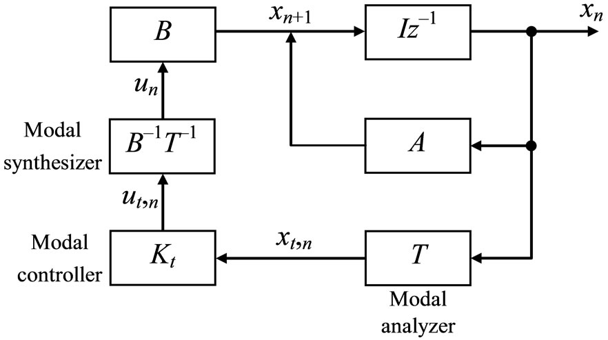
Figure 1. Block diagram of system with modal control.
relationships given below were taken from [7].
The system is described by the following difference equation
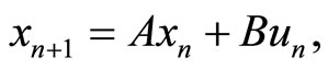 (36)
(36)
where xn, un, А, and В are k-size state vector, control vector, system matrix, and input matrix, respectively, n = 0, 1, 2, ···
A transformation with the help of a nonsingular matrix T
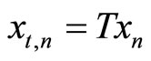 (37)
(37)
gives Equation (36) in the form
 (38)
(38)
where Λ = ТАТ–1, ut,n = Вtun, and Вt = ТВ, with a diagonal matrix.
Constructing the control in the form of a feedback on a vector of variables with a diagonal matrix
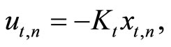 (39)
(39)
performed by the modal analyzer, one leads to the homogeneous equation
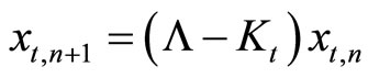 (40)
(40)
with a diagonal matrix. This enables one to control each of eigenvalues by means of changing a one element of the matrix (39).
A modal synthesizer rebuilds the real control vector according to the Equations (38) and (39)
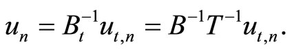
The method offered here, as well as the Frobenius transformation, allows a separate eigenvalue to be controlled by changing not a single but all of k elements in row or column, and also if they are arbitrarily selected. As it was noted, practical interest is the case of change in row elements. This case belongs to the class of the most widespread control systems with a unique control input.
The block diagram of a modal control system with a unique input shown in Figure 2 does not include blocks providing a transformation of variables. Here, the modal controller represents a set of two-input products, each of which performs multiplication of a state variable by a feedback coefficient. The sum of multiplication results goes to the input.
In this case, Equation (36) takes the form
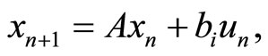 (41)
(41)
where bi is a vector with all zero elements except i-th element that is a one. This element defines the input number.
The feedback , where K is a vector of coefficients, gives the equation in the form of (40)
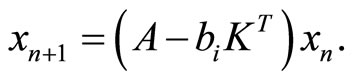 (42)
(42)
The row KT is calculated as the i-th row of a summary matrix G of the row supplements of the LST. As a result, we obtain a matrix in (42) with a desirable spectrum.
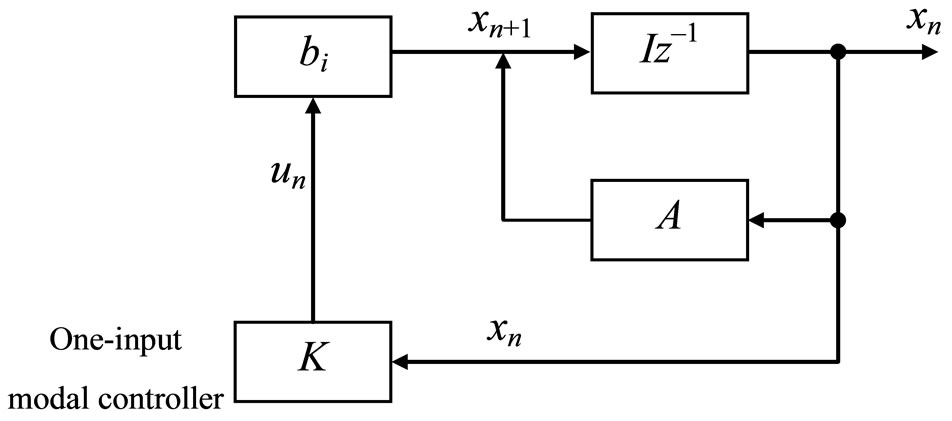
Figure 2. Block diagram of system with one-input modal control.