Applied Mathematics
Vol.3 No.12(2012), Article ID:25344,6 pages DOI:10.4236/am.2012.312253
Iterative Solution Methods for a Class of State and Control Constrained Optimal Control Problems
1University of Oulu, Oulu, Finland
2Kazan Federal University, Kazan, Russia
Email: erkki.laitinen@oulu.fi
Received September 1, 2012; revised October 11, 2012; accepted October 18, 2012
Keywords: Constrained Optimal Control Problem; Saddle Point Problem; Finite Element Method; Iterative Algorithm
ABSTRACT
Iterative methods for solving discrete optimal control problems are constructed and investigated. These discrete problems arise when approximating by finite difference method or by finite element method the optimal control problems which contain a linear elliptic boundary value problem as a state equation, control in the righthand side of the equation or in the boundary conditions, and point-wise constraints for both state and control functions. The convergence of the constructed iterative methods is proved, the implementation problems are discussed, and the numerical comparison of the methods is executed.
1. Sample Examples of the State and Control Constrained Optimal Control Problems
We give two sample examples of the elliptic optimal control problems. The corresponding existence theory, methods of the approximation and more examples can be found, e.g., in [1,2] (see also the bibliography therein).
Consider the homogeneous Dirichlet boundary value problem for Poisson equation which plays a role of the state problem in first sample example:
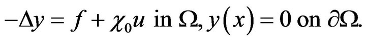 (1)
(1)
Above  is a bounded domain with piecewise smooth boundary
 ,
,  is the characteristic function of a subdomain
 ,
,  is a fixed function, while
 ![]() is a variable control function. For all
is a variable control function. For all  there exists a unique weak solution
 ![]() of the boundary value problem (1) from Sobolev space
of the boundary value problem (1) from Sobolev space . We impose the point-wise constraints for both state function
 ![]() and control function
and control function![]() :
:
 (2)
(2)
with  and
and 
Suppose that (1) and (2) are not contradictory in the sense that
 (3)
(3)
Let the objective functional be defined by the equality

with a given function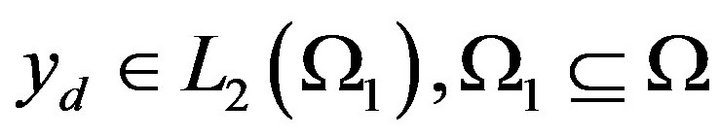 . The optimal control problem
 (4)
(4)
has a unique solution  if assumption (3) is fulfilled.
In the second sample example we take as the state problem mixed boundary value problem for Poisson equation
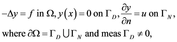 (5)
(5)
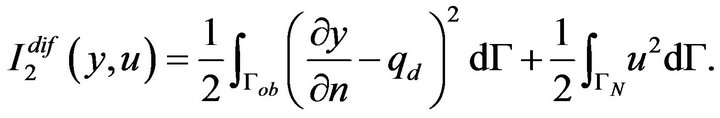
and the objective functional of the form
Here ![]() is the unit vector of outward normal,
is the unit vector of outward normal,  and
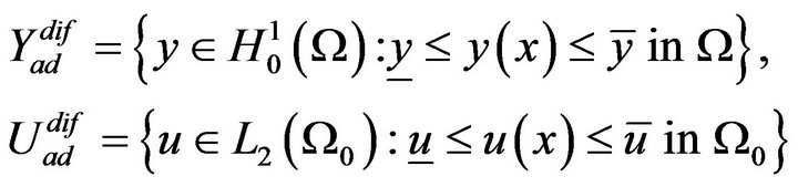
and  Let the constraints for
 ![]() and
and ![]() be
be
Suppose again that the set

is not empty. Then the optimal control problem
 (6)
(6)
has a unique solution .
.
2. Finite Element Approximation of the Optimal Control Problems
We briefly describe the approximation of the problems (4) and (6) by a finite element method (cf. [3]). Suppose that the domains ,
,  and
and  are polygons and construct a conforming triangulation of
  into triangle and/or rectangle finite elements
![]() . Let the triangulation be consistent with the subdomains
. Let the triangulation be consistent with the subdomains  and
and  and the partition of the boundary into the parts
 ,
,  and
and  in the following sense: every subdomain consists of the integer number of the elements
 ![]() and every part of the boundary consists of the integer number of the sides of
and every part of the boundary consists of the integer number of the sides of![]() . Construct the finite element spaces which consist of the continuous functions, piecewise linear on the triangles (
. Construct the finite element spaces which consist of the continuous functions, piecewise linear on the triangles ( -elements) and piecewise bilinear on the rectangles (
 -elements), and satisfy Dirichlet boundary conditions. The integrals over domains and curves we approximate by the composed quadrature formulaes using the simplest 3-points quadrature formulaes for the triangle elements
 ![]() and 4-points formulaes for the rectangle elements
and 4-points formulaes for the rectangle elements![]() . Note, that such kind of the approximation of a 2nd order elliptic equation in the case of rectangular
. Note, that such kind of the approximation of a 2nd order elliptic equation in the case of rectangular  and rectangular elements
 ![]() coincides with a finite difference approximation of this equation.
coincides with a finite difference approximation of this equation.
We apply the described above approximation procedure for the sample optimal control problems and obtain the mesh optimal control problems which are the finite dimensional problems for the vectors of nodal values1 of the corresponding mesh functions. Namely, the approximations of the state problems (1) and (5) are the discrete state equations of the form
where  is a positive definite stiffness matrix,
  is a diagonal mass matrix, and
 is a rectangular matrix. The discrete objective function approximating
  or
or  is a quadratical function
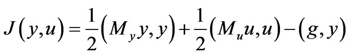
with a symmetric and positive definite matrix  , symmetric and positive semidefinite matrix
 , and given vector
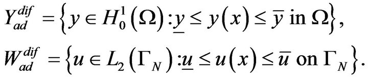
 . Finally, the sets of constraints for the vectors
 ![]() and
and ![]() are
are

Further we denote by 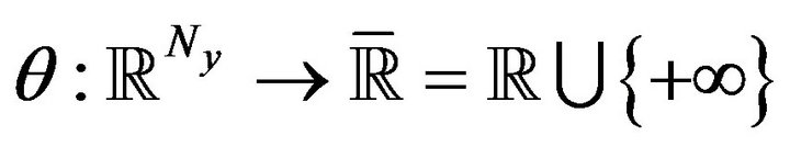 and
and 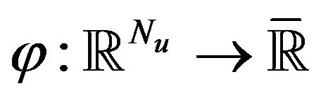 the indicator functions of the sets
  and
and , respectively. Resulting mesh optimal control problem which approximates (4) or (6) can be written in the following form:
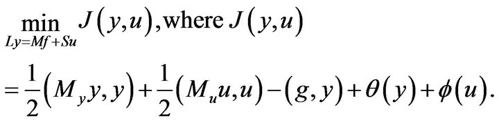 (7)
(7)
Below we list the main properties of the matrices and functions in problem (7) which are used for its theoretical investigation and proving the convergence of the corresponding iterative methods:
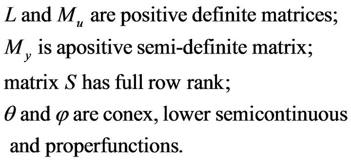 (8)
(8)
Minimization problem (7) with the matrices and the functions which satisfy assumptions (8) arise when approximating by finite difference method or by simplest finite element methods with quadrature formulaes the wide class of the optimal control problems which contain a linear boundary value problem as a state equation, control in the right-hand side of the equation or in the boundary conditions, and point-wise constraints for both state and control functions.
Introduce Lagrange function for problem (7):

Its saddle point  satisfies the saddle point problem
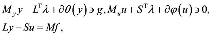 (9)
(9)
where  and
and  are the subdifferentials of the corresponding functions.
Theorem 1 Let the assumptions (8) be valid and
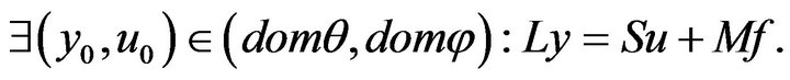
Then problem (7) has a unique solution . If more strict assumption

is fulfilled then saddle point problem (9) has a nonempty set of solutions .
.
3. Transformations of the Primal Saddle Point Problem and Preconditioned Uzawa Method
Matrix  which multiplies by the vector
 in system (9) is only positive semidefinite. This prevents the usage of the dual iterative methods (such as Uzawa method) for solving (9). We transform this saddle point problem to an equivalent one with a positive definite matrix by using the last equation in system (9). Consider two equivalent to (9) saddle point problems:
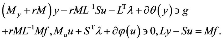 (10)
(10)
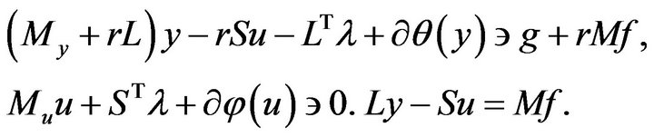 (11)
(11)
Lemma 1 Matrices  and
and
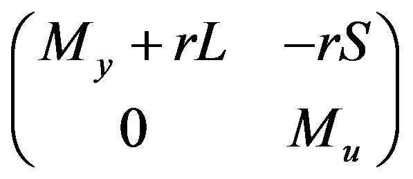 are positive definite for
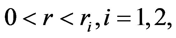 where constants
  don’t depend on the dimension of the finite element space (or, on the mesh step).
Now, we can apply the preconditioned Uzawa methods for solving problem (10) and problem (11):
 (12)
(12)
 (13)
(13)
The choice of the preconditioners is based on the properties of the matrices in problems (10) and (11) (see the corresponding theory in [4]).
Lemma 2 The iterative methods (12) and (13) converge if , where
 ![]() don’t depend on mesh step.
don’t depend on mesh step.
The implementation of every step of (12) includes solution of two systems of linear equations with matrices ![]() and
and  and solution of two inclusions with multivalued operators
  and
and . The matrices in the discrete model problems are diagonal while the functions are separable:
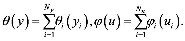
Due to these properties  and
and  are diagonal operators, and the solution of the inclusions with these operators reduce to an easy problem of the orthogonal projection on the corresponding sets
  and
and .
.
The implementation of every step of (13) includes solution of the system of linear equations with matrix  and solution of the inclusion with operator
 , which corresponds to a mesh variational inequality of second order. This is more time consuming problem than solution of a linear system, but the numerical tests demonstrates the preference of method (13) in some particular cases. The methods of solving the variational inequalities can be found in the books [5-7].
4. Block SOR-Method for the Problem with Penalization of the State Equation
Let D be a symmetric and positive matrix while  be a regularization parameter. Consider the following regularization of problem (7):
 (14)
(14)
Theorem 2 Let the assumptions (8) be valid. Then problem (14) has a unique solution  If
If  is a solution of saddle point problem (9), then the following estimate holds:
 (15)
(15)
with a constant ![]() independent on
independent on ![]() and on mesh size.
and on mesh size.
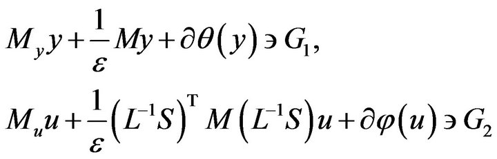
Problem (14) is equivalent to the following system of the inclusions:
 (16)
(16)
with a positive definite and symmetric matrix. Different iterative methods can be used for solving problem (14) or equivalent problem (16) (see, e.g., [5,6] and the bibliography therein). We solve system (16) by block SORmethod:
 (17)
(17)
where  is a relaxation parameter and

Theorem 3 ([8]) Method (17) converges for any .
.
The implementation of (17) depends on the choice of the matrix . Below we consider two variants of the choice.
a) Let . In this case the implementation of every iterative step of (17) consists of the solving the following system
 (18)
(18)
with known . For the model problems under consideration the operator
  of the first inclusion has diagonal form, so, its solution reduces the projection on the set
 . Further, the matrix in the second inclusion is spectrally equivalent to matrix
 :
:
Here  is a constant in the stability estimate for a solution of the state equation and it is independent on mesh step. The stationary one-step iterative method with preconditioner
  converges with the rate of convergence proportional to
 ![]() (and doesn’t depend on mesh step), and its implementation reduces to the projection on the set
(and doesn’t depend on mesh step), and its implementation reduces to the projection on the set .
.
In the particular case when ![]() is the unit matrix (which corresponds to the distributed in the domain control) the second inclusion in (18) can be transformed to a system of nonlinear equations and an inclusion with diagonal operator. Namely, let
is the unit matrix (which corresponds to the distributed in the domain control) the second inclusion in (18) can be transformed to a system of nonlinear equations and an inclusion with diagonal operator. Namely, let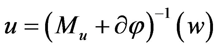 . Then the auxiliary vector
 ![]() is a solution of the system of nonlinear algebraic equations
is a solution of the system of nonlinear algebraic equations
with the symmetric and positive definite matrix
 and monotone, diagonal and Lipshitz-continuous operator
 .
.
b) In the case of a symmetric matrix ![]() and the unit matrix
and the unit matrix ![]() the promising choice is
the promising choice is . Then on every iterative step of (17) we solve the system

First inclusion of this system corresponds to a mesh approximation of a second order variational inequality, while the equation for vector ![]() contains the symmetric and positive matrix
contains the symmetric and positive matrix ![]() and monotone, diagonal and Lipshitz-continuous operator
and monotone, diagonal and Lipshitz-continuous operator .
.
5. Numerical Example
We solved the optimal control problem with the following state problem and constraints:

and the objective functional

where  and
and .
.
Finite difference approximation of this optimal control problem on the uniform grid leads to a minimization problem of the form (7) and the following saddle point problem (particular case of (9)):

Here symmetric and positive definite matrix ![]() corresponds to the mesh Laplacian with Dirichlet boundary conditions,
corresponds to the mesh Laplacian with Dirichlet boundary conditions,  is a diagonal and positive semidefinite matrix (its positive entries correspond to the grid points in the subdomain
 ).
).
To apply Uzawa method we used the equivalent transformation similar to (11) with parameter  (satisfying the assumptions of theorem 1):

This system was solved by Uzawa method with preconditioner ![]() which is now spectrally equivalent to
which is now spectrally equivalent to .
.
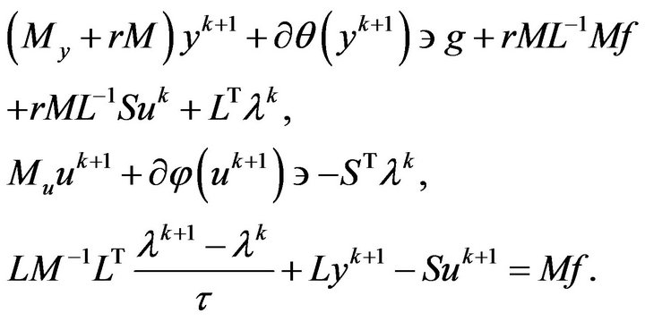
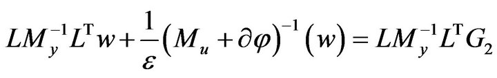
We also solved the mesh optimal control problem by applying SOR-method to the problem with penalized state equation and the choice . Corresponding system for
![]() ,
, ![]() and auxiliary vector
and auxiliary vector ![]() reads as:
reads as:
We used block SOR-method with relaxation parameter  (found numerically to be close to optimal one). We also used the iterative regularization as follows: calculate the residual vector
  on the current iteration
and set  when
when  becomes less than 1.
Here the norm  is the mesh analogue of the Lesbegue space norm
 . The smallest value
  was reached started from
 .
.
In the tables below (Tables 1 and 2)  is the number of an iteration,
  is the value of the objective function on the current iteration,
  and
and
 , the calculation results for the
are presented. We constructed the exact solution  of the discrete optimal control problem, so, we knew the exact minimum of the cost function
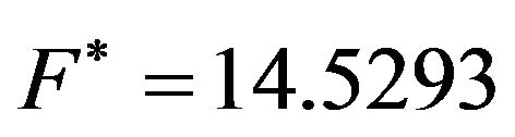 .
.
We can conclude that block SOR method had a big advantage in comparison with preconditioned Uzawa method in the accuracy of the calculated state y and control![]() .
.
A number of calculations were made for the different state and control constrained optimal control problems on the different meshes. All of them demonstrated the pref-
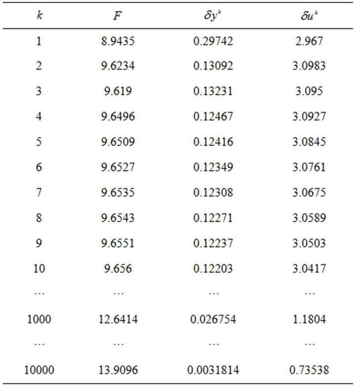
Table 1. Uzawa method.
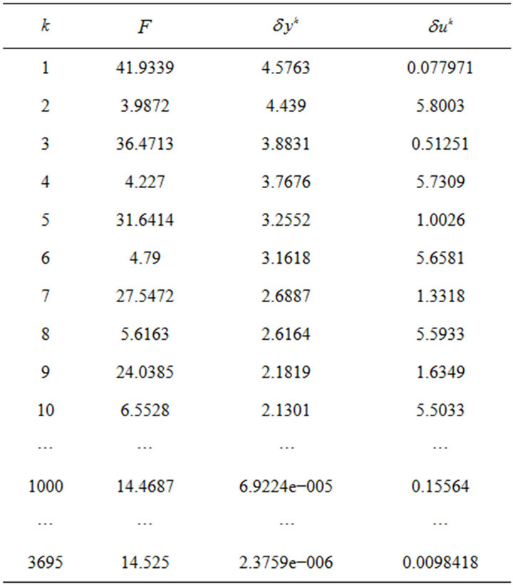
Table 2. Block SOR method.
erence of the iterative methods based on the penalty of the state equation in the comparison with the preconditioned Uzawa methods, while that were faster convergent than the gradient methods applied for the problems with the penalization of the state constraints (see [9,10]).
REFERENCES
- J.-L. Lions, “Optimal Control of Systems Gouverhed by Partial Differential Equations,” Springer-Verlag, New York, 1971. doi:10.1007/978-3-642-65024-6
- P. Neittaanmaki, J. Sprekels and D. Tiba, “Optimization of Elliptic Systems. Theory and Applications,” SpringerVerlag, New York, 2006.
- P. H. Ciarlet and J.-L. Lions, “Handbook of Mumerical Analysis: Finite Element Methods,” North-Holland, Amsterdam, 1991.
- A. Lapin, “Preconditioned Uzawa-Type Methods for Finite-Dimensional Constrained Saddle Point Problems,” Lobachevskii Journal of Mathematics, Vol. 31, No. 4, 2010, pp. 309-322.
- R. Glowinski, J.-L. Lions and R. Tremolieres, “Numeral Analysis of Variational Inequalities,” Translated and Revised Edition, North-Holland Publishing Company, Amsterdam, New York and Oxford, 1981.
- A. Lapin, “Iterative Solution Methods for Mesh Variational Inequalities,” Kazan State University, Kazan, 2008.
- I. Hlavacĕk, J. Haslinger, J. Necăs and J. Lovisĕk, “Solution of Variational Inequalities in Mechanics,” Springer Verlag, New York, 1988.
- A. V. Lapin, “Methods of Upper Relaxation Type for the Sum of a Quadratic and a Convex Functional,” Izvestiya Vysshikh Uchebnykh Zavedenii. Matematika, No. 8, 1993, pp. 30-39.
- A. Lapin and M. Khasanov, “State-Constrained Optimal Control of an Elliptic Equation with Its Right-Hand Side Used as Control Function,” Lobachevskii Journal of Mathematics, Vol. 32, No. 4, 2011, pp. 453-462. doi:10.1134/S1995080211040287
- E. Laitinen and A. Lapin, “Iterative Solution Methods for the Large Scale Constrained Saddle Point Problems,” In: S. Repin, T. Tiihonen and T. Tuovinen, Eds., Numerical Methods for Differential Equations, Optimization, and Technological Problems, Springer, New York, 2012, pp. 19-39.
NOTES
1Hereafter we use the same notations y, u for the vectors and for the functions in the differential problems. This doesn’t lead to a confuse because later we consider only finite-dimensional problems.