Journal of Electromagnetic Analysis and Applications
Vol.4 No.2(2012), Article ID:17670,8 pages DOI:10.4236/jemaa.2012.42009
Quasi-Dynamic Green’s Functions for Efficient Full-Wave Integral Formulations for Microstrip Interconnects
![]()
1D.I.I., Second University of Naples, Aversa, Italy; 2D.I.E.I., University of Cassino and Southern Lazio, Cassino, Italy.
Email: *maffucci@unicas.it
Received December 22nd, 2011; revised January 20th, 2012; accepted January 29th, 2012
Keywords: Full-Wave Models; Green’s Function; Integral Formulations; Microstrip Interconnects
ABSTRACT
Integral formulations are widely used for full-wave analysis of microstrip interconnects. A weak point of these formulations is the inclusion of the proper planar-layered Green’s Functions (GFs), because of their computational cost. To overcome this problem, usually the GFs are decomposed into a quasi-dynamic term and a dynamic one. Under suitable approximations, the first may be given in closed form, whereas the second is approximated. Starting from a general criterion for this decomposition, in this paper we derive some simple criteria for using the closed-form quasi-dynamic GFs instead of the complete GFs, with reference to the problem of evaluating the full-wave current distribution along microstrips. These criteria are based on simple relations between frequency, line length, dielectric thickness and permittivity. The layered GFs have been embedded into a full-wave transmission line model and the results are first benchmarked with respect to a full-wave numerical 3D tool, then used to assess the proposed criteria.
1. Introduction
Full-wave analysis of high-speed interconnects is challenging both in problem formulation and in computational efficiency. In these structures the conductors fill a limited region of space, and thus integral approaches to Maxwell equations are widely used, e.g., [1-6]. A popular approach for numerical solution of integral equations is the Method of Moments [3]. Integral formulations have main advantages: 1) the limited discretization region, which reduces to the conductor volumes or sometimes the conductor surfaces; 2) the possibility to rigorously impose the regularity conditions at infinity. On the contrary, differential approaches require the solution in the overall domain, a suitably large but finite box, where the regularity conditions are approximately imposed.
For Integrated Circuit (IC) and Printed Circuit Board (PCB) simulation, the electromagnetic analysis is only the first step, usually followed by a further step of derivation of equivalent circuits. A successful example of this approach is given by the popular Partial Element Equivalent Circuit (PEEC) method [4].
A weak point of integral formulations is the non-trivial inclusion of inhomogeneous dielectrics. There are two possible ways to face such a problem. A simplified approach consists in deriving an effective dielectric constant, and keep on using the Green’s functions (GFs) for homogeneous media. An example of definition of effective permittivity is given in [6]. The second approach is the use of the GFs for inhomogeneous media, starting from their expression in the spectral domain. In such a domain it is possible to give closed form expressions to GFs, when considering planar, cylindrical and spherical layered media [7,8]. The corresponding GFs in the spatial domain are expressed in terms of Sommerfeld integrals. The slow decaying nature of the integrands and the oscillatory nature of the Sommerfeld integrals make the numerical integration extremely slow and dramatically increases the computational cost of any numerical model based on integral formulation. For this reason, the efficient evaluation of the GFs has gained the attention of literature over the years, and still poses open questions, e.g., [9-15].
The most efficient approaches in literature are based on the semi-analytical evaluation of the so-called quasidynamic term of the frequency domain GFs. The remainders are then fitted by means of different approximation methods. Some criteria are also proposed to establish when the complete GFs are satisfactorily approximated by the quasi-dynamic terms.
In this paper the GFs decomposition is used with reference to a particular class of problems, namely the evaluation of the full-wave current distributions along coupled microstrips. This means that planar layered media are considered. A brief review of the integral formulation of the electromagnetic signal propagation along a microstrip is given in Section 2. A full-wave transmission line model for microstrips is also recalled, which is here implemented using both the complete and the approximated GFs. To this purpose, some of the most popular techniques for GFs decomposition are reviewed in Section 3. Using the proposed model, in Section 4 simple criteria are derived to establish when it is possible to replace the complete GF with the quasi-dynamic GF.
2. Full-Wave Transmission Line Model
The reference problem analyzed here (Figure 1) is a coupled microstrip structure, where two or more signal traces, in general with different widths, are placed on a dielectric plane of thickness t, above a PEC ground plane. The conductors and dielectrics are assumed ideal. In the following, we review the main features of an integral formulation for modeling such a structure, and a semianalytical full-wave model derived from this formulation.
2.1. Electric Field Integral Equation
In the so-called Electrical Field Integral Equation (EFIE) formulation, the electric field E is expressed in terms of scalar and vector potentials [2]:
 (1)
(1)
and the potentials are related to the “sources” (the current density J and charge density ) through the integrals:
 (2)
(2)
 (3)
(3)
whose kernels involve the Green’s functions (GFs) of the considered structure. The integration domain V is the region where the sources are located, which could be a volume or a surface, depending on the application. In the general case, the GF for the vector potential,  , is dyadic, whereas the GF for the scalar potential,
  , is a scalar. In free space it is:
 (4)
(4)
being I the identity matrix, and k0 the vacuum space wavenumber.
In principle, a rigorous full-wave simulation should take into account the 3D nature of the structure: this approach leads to a prohibitive computational cost when a realistic PCB board is considered. However, when the second order effects due to the finite size dimensions of the board can be neglected, the dielectric substrate can be considered infinite in the x-y plane and layered in the z direction, e.g. [16,17]. Under this hypothesis, it is possible to give a closed form expression to the GFs in the spectral domain, which will be denoted in the following with  and
and , e.g., [9-12]. The spatial domain GFs are obtained as solutions of the following Sommerfeld integrals:
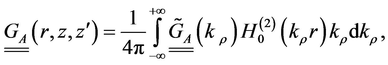 (5)
(5)
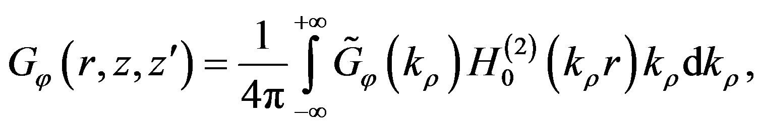 (6)
(6)
where  is the Hankel function of second kind and order 0, r is the distance in the plane xy, z and z′ are, respectively, the horizontal positions of the observer and the source. The integration path lies in the first and third quadrant of the kρ—complex plane, and detours around the poles and the branch point of the argument.
A brute force numerical computation of Sommerfeld integrals is time consuming, due to the slow decaying nature of the integrands.
2.2. Full-Wave Transmission Line Model
Semi-analytical full-wave transmission line (TL) models are proposed in literature to catch high-frequency effects like dispersion related to finite size [17-19] or losses associated to spurious radiation [20,21]. In this paper we use a generalized TL model, derived from the EFIE formulation presented in 2.1. This model, the Enhanced Transmission Line (ETL) model, has been derived in [17-20], assuming geometrically long line, electrically short conductor thickness and uniform cross sections.
Let us introduce the vectors of currents, voltages, perunit-length (p.u.l.) magnetic flux and p.u.l. charge, with the typical references used in TL models. The ETL equations in frequency domain are [17-20]:
 , (7)
, (7)
 (8)
(8)
 . (9)
. (9)
Here the matrix kernels HI and HQ are expressed in terms of the GFs: their generic entry is given by:
 (10)
(10)
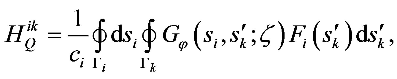 (11)
(11)
where Γi is the contour of the i-th conductor in the cross-section, ci its length and si the curvilinear abscissa. The function Fi describes the distribution of the sources along Γi, in the static limit.
The classical TL model is derived assuming low frequency and infinitely long line, so that (8) and (9) reduce to the well-known relations:
 (12)
(12)
being L and C the classical p.u.l. inductance and capacitance matrices. The main difference between the classical TL model and the ETL one is the non-local relations imposed by (8) and (9). If k is the wavenumber and t the characteristic transverse dimension of the interconnect, the classical TL model is valid for , (typically for kt up to 0.1), whereas the ETL model may be used up to
  [17-20]. The computational cost of this model is given by the cost of a TL model, augmented by the cost of integrals (8) and (9), which is strongly affected by the cost of the GFs evaluation.
3. Efficient Evaluation of the Green’s Functions
3.1. Green’s Functions Decomposition and Quasi-Dynamic Term
A way to lower the computational cost of the Sommerfeld integrals is to approximate the spectral domain GFs in terms of functions for which such integrals are analytically known. The GFs are decomposed into a quasidynamic and a dynamic part:
 . (13)
The quasi-dynamic term,  , is the asymptotic value in the limit
 . The corresponding spatial domain term
  dominates the near field interaction (
 ), i.e. the low frequency and low distance ranges. Let us consider the components
  and
and  of the spatial domain GFs. For the microstrip analyzed here, these are the only components of interest, when z > 0 and z′ > 0. In the limit
 , these components may be obtained in closed form [9-15]. Let us introduce:
 (14)
(14)
 (15)
(15)
 (16)
(16)
where  In the spectral domain the quasidynamic GFs may be expressed in closed form as:
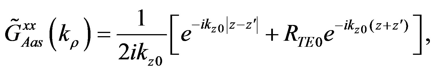 (17)
(17)
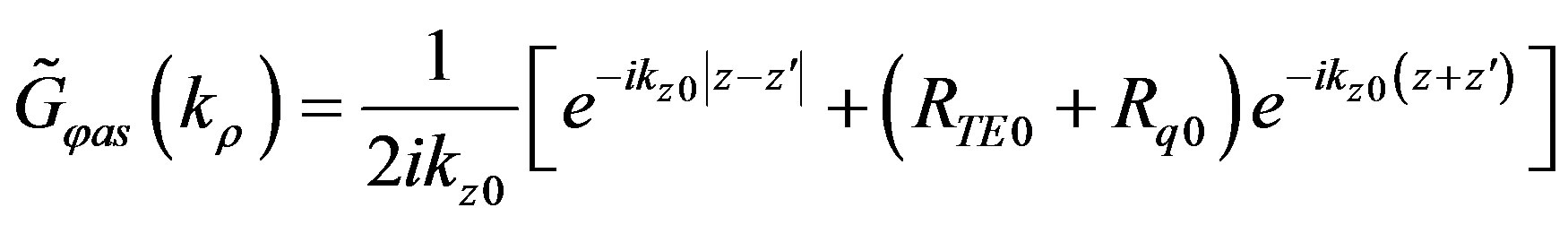 (18)
(18)
which correspond in the spatial domain to:
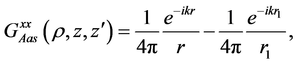 (19)
(19)
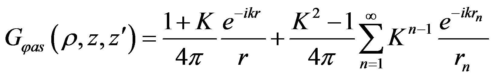 (20)
(20)
where
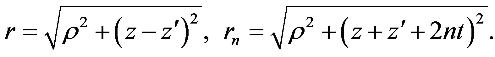 (21)
(21)
3.2. Approximation of the GF Dynamic Terms
Let us now investigate the dynamic part  in (13), which is the dominating term in the far-field region and describes phenomena like surface waves or, more generally, waves associated to the continuous spectrum. This cannot be given in closed form and must be approximated. In the following, we briefly recall three of the most used approaches to this problem.
In the Discrete Complex Image Method (DCIM), the dynamic part  is approximated by the sum of a series of complex exponentials and a term describing the TM/TE surface waves [9,22]:
 (22)
(22)
where  and
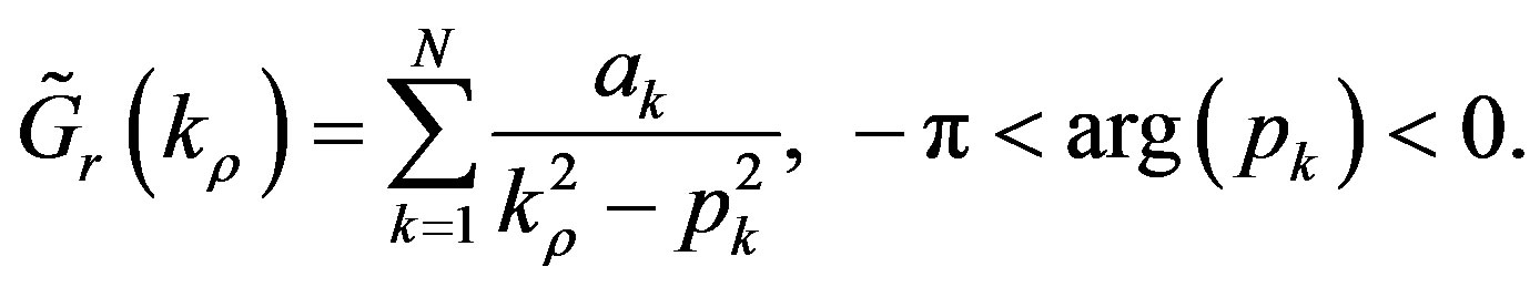
and  are, respectively, the residuals and the poles of the TE and TM surface waves. This technique suffers from a time-consuming poles-residues extraction. Furthermore, a large number of images is needed to achieve a good accuracy. A more suitable approach is the so-called Rational Fitting Function Method (RFFM), which is based on the approximation of the dynamic part in terms of rational functions using the robust identification algorithm Vector Fitting [12]:
 (23)
(23)
This leads in the spatial domain to a series of cylindrical waves:
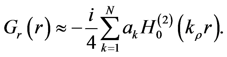 (24)
(24)
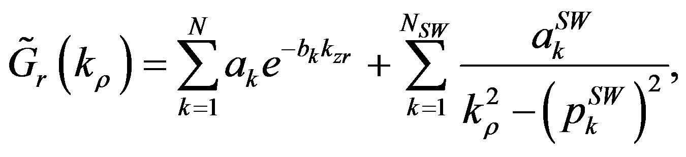
This technique is very efficient since the Vector Fitting provides few poles. However, the use of Hankel functions without any constrain may lead to same nonphysical singularities for  with
with  (note that the same problem occurs for DCIM). This problem is solved with the Total Least Square Method (TLSM), where the dynamic part
  is expressed as a fraction of two polynomials [15]:
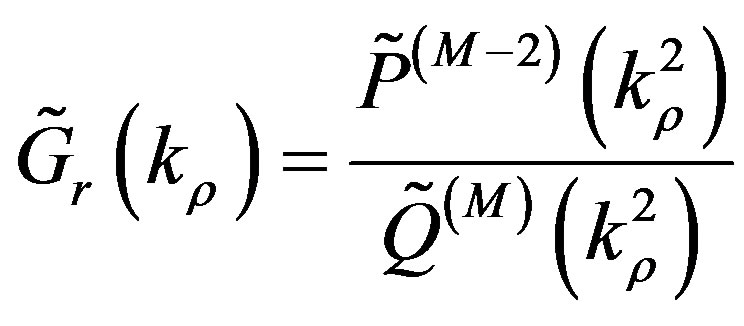 (25)
(25)
where  and
and  are polynomials of degrees M − 2 and M, respectively. The poles and residues of (25) are extracted using the Total Least Square Technique, leading to the same approximated structure as in (23), corresponding to (24) in the spatial domain. This technique provides a number of poles even lower than the RFFM one, and avoids the problem of the non-physical singularities, since
  for
for 
3.3. Computational Cost and Truncation Criteria
Whatever is the method used to approximate the GFs, the above results yield to an increase of complexity of the layered media GFs, compared to the free-space one (4). The quasi-dynamic term of GF (20) is usually approximated by 2 - 3 few spherical waves. The approximation (24) of the dynamic term requires around 10 cylindrical waves (Hankel functions). Assuming that the computational cost of a cylindrical wave is comparable to that of a spherical one (which is an optimistic case), the evaluation of the approximated dynamic parts of the GFs would cost at least 50 times the cost of the free-space GF. For this reason, the definition of truncation criteria for these approximated parts of the GFs is of great interest.
The computational cost may be dramatically reduced when the GFs reduce to the quasi-dynamic terms, known in closed form. This happens when the following criteria are satisfied [9]:
 (26)
(26)
remembering that  is the distance between the source and the field point in the plane x-y.
4. Full-Wave Analysis of Microstrips
The general results obtained in Section 3 are here applied to full-wave analysis of microstrips, assuming the reference structure in Figure 1, with w1 = 0.25 mm, w2 = 0.50 mm, w = 0.228 mm, t = 0.60 mm and εr = 4.4.
Green’s Functions Evaluation for Microstrips
Let us investigate the application of conditions (26) to the considered structure. Figures 2 and 3 show, respectively, the scalar potential and the vector potential GFs, computed at 0.1 GHz. At such a frequency it is 
 , hence the first of (26) is satisfied. The results confirm also the validity of the second of (26). Note that the vector potential GF is quite insensitive to the second of conditions (26). Figures 4 and 5 refer to a frequency
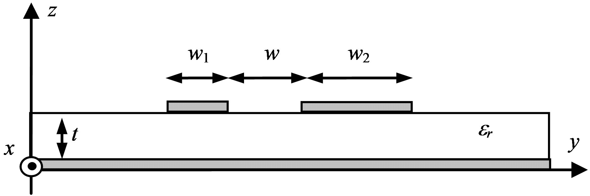
Figure 1. The analyzed microstrip structure.
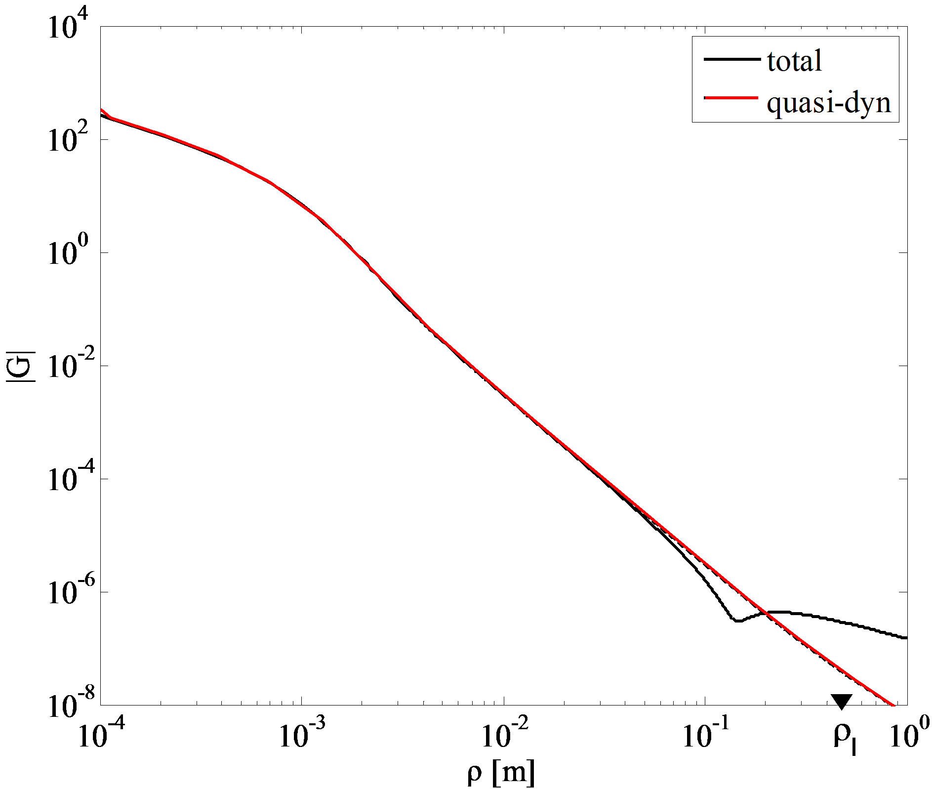
Figure 2. Scalar potential Green’s function, computed at 0.1 GHz.
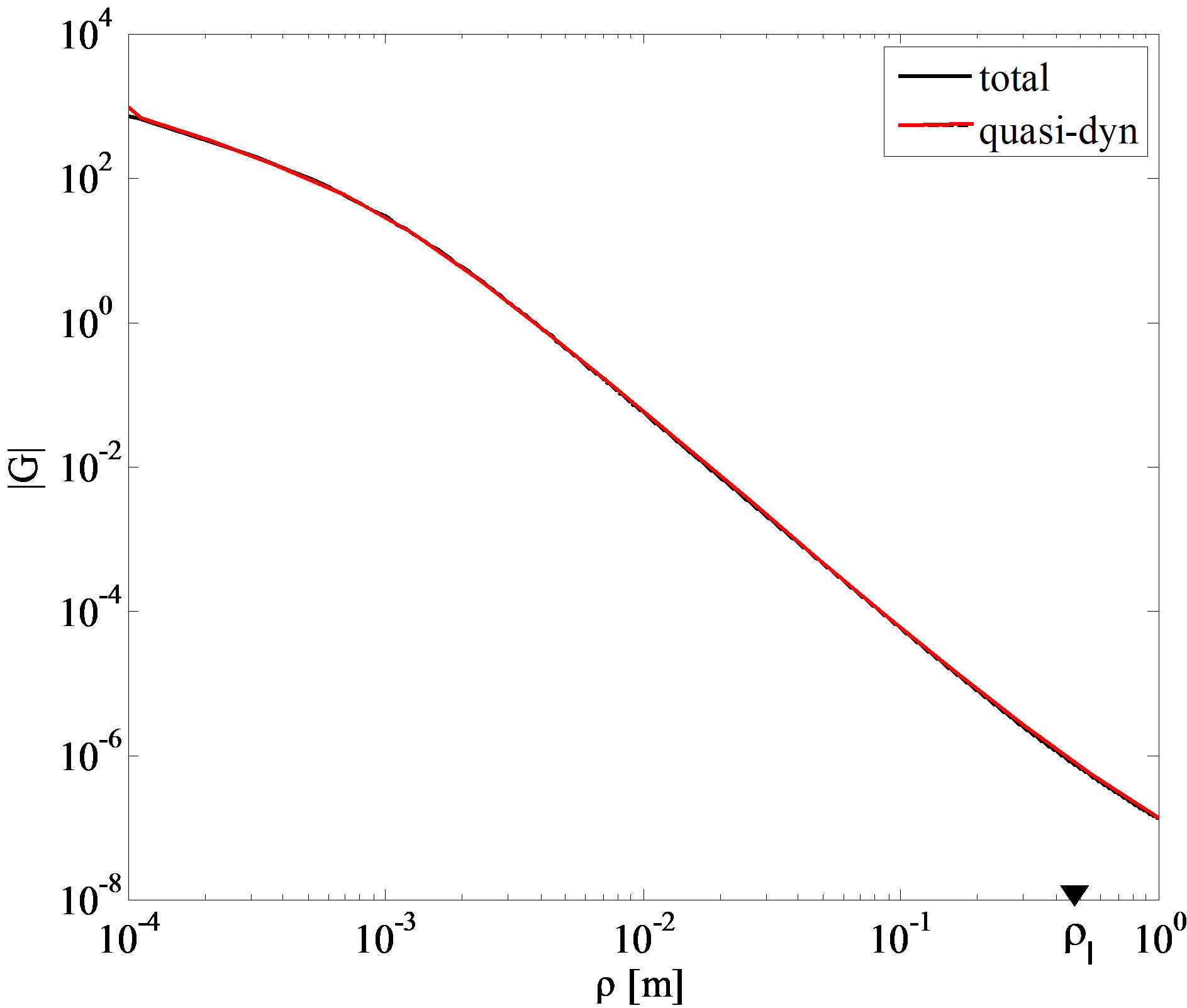
Figure 3. Vector potential Green’s function, computed at 0.1 GHz.
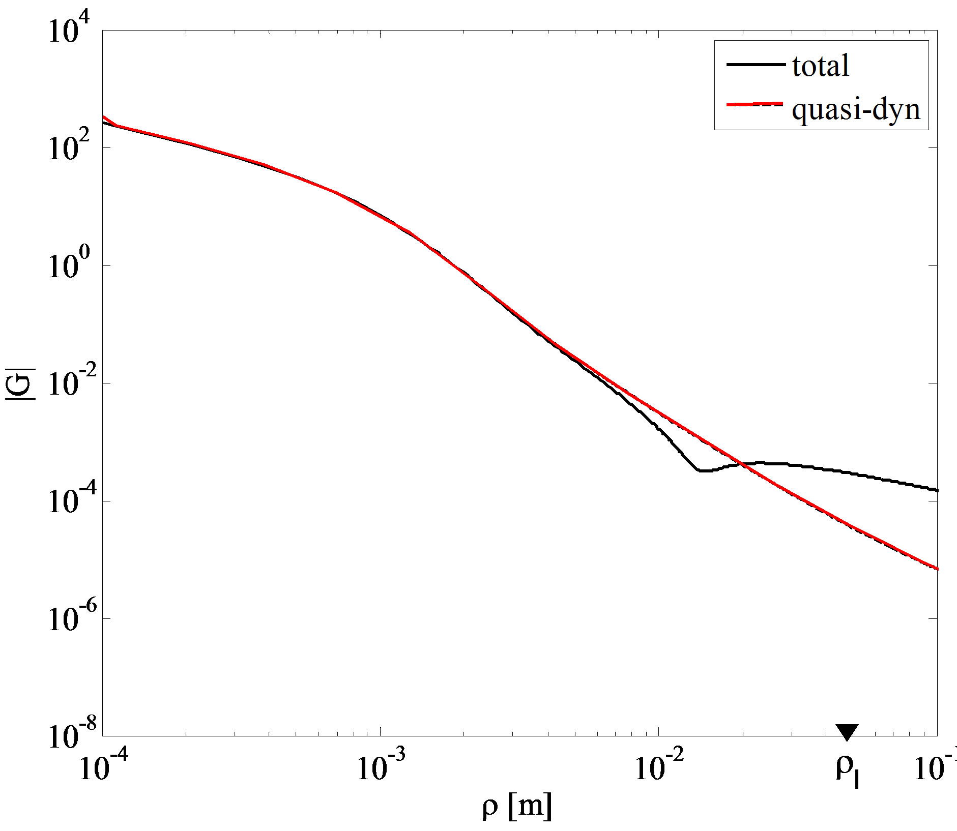
Figure 4. Scalar potential Green’s function computed at 1 GHz.
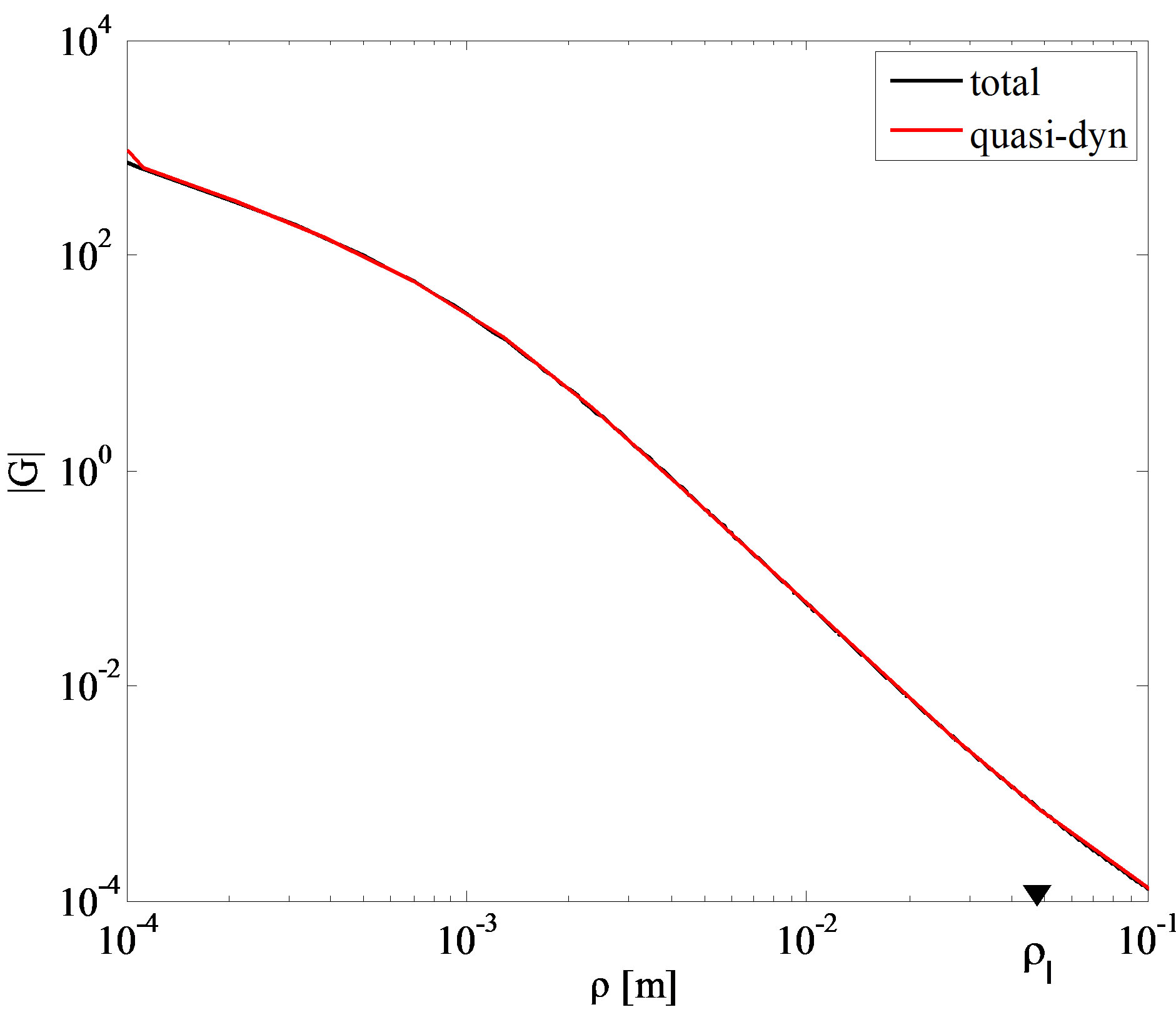
Figure 5. Vector potential Green’s function computed at 1 GHz.
of 1 GHz, hence to .
.
As shown in these figures, for increasing frequency, the parameter b decreases, and so the quasi-dynamic terms approximate the complete GFs for lower distances.
In the following, we will derive from (26) some criteria which are directly applicable to the class of problems of guided propagation, such as the microstrips. Our target here is the evaluation of the full-wave current distributions along the microstrip traces, obtained by means of the ETL model presented in Section 2. Here we assume that the coupled microstrip is fed at one end by a differential current of amplitude 1 [a.u], and left open at the other end.
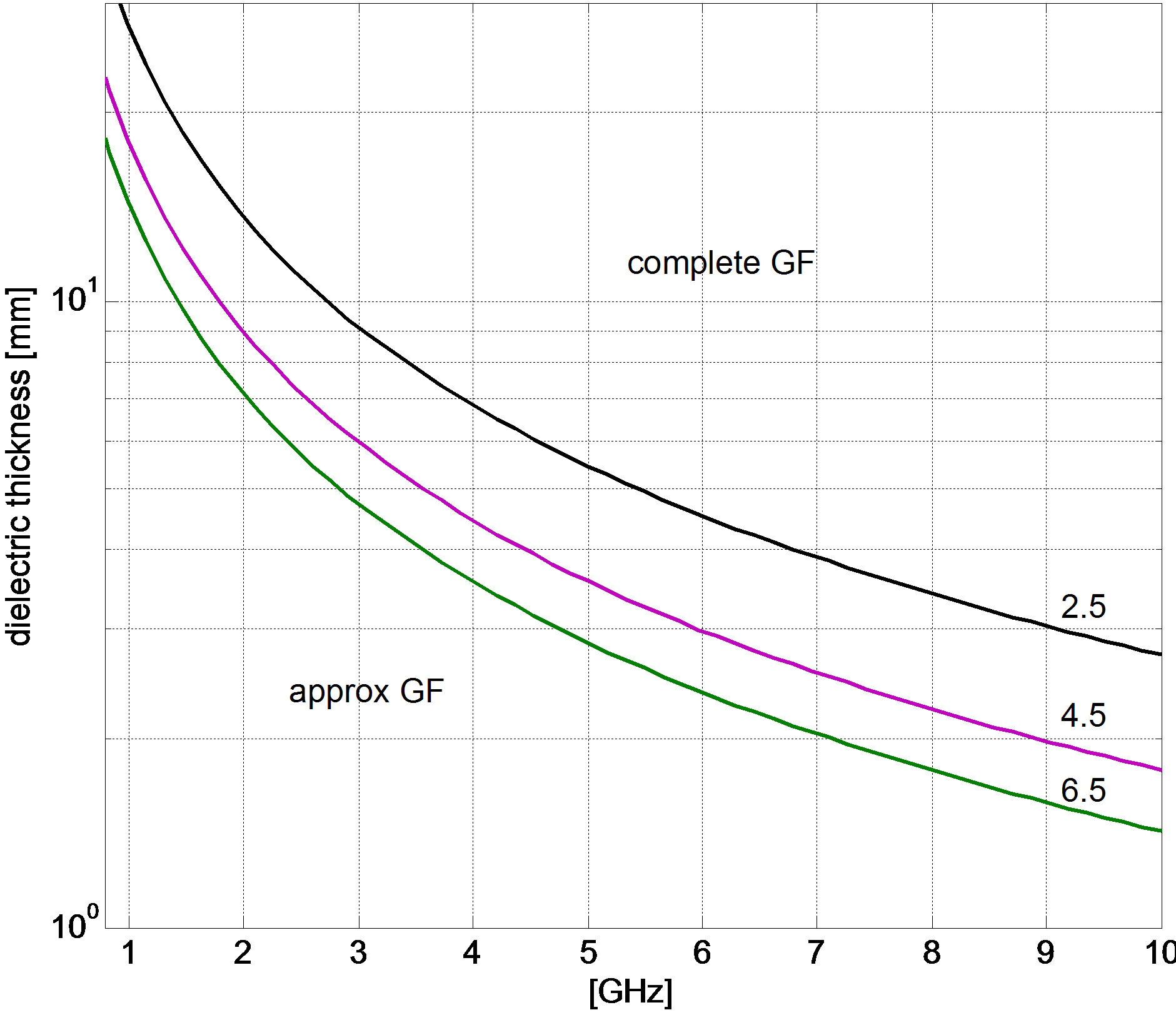
Let us apply the general criteria (26) to this class of problem. First we assume , being len the line length. Figures 6 plot the maps obtained from criteria (26), assuming three different values for the dielectric permittivity. Figure 6(a) plots the dielectric thickness versus frequency: the region where the approximated GFs may be used falls below the curve corresponding to the chosen permittivity value. Figure 6(b) shows, instead, the map given by the second of (26), assuming again
 : the line length is plotted versus frequency. The above conditions are summarized in Figure 7, where a map showing both the geometrical parameters is plotted. These parameters are normalized to the wavenumber, therefore the map is independent from frequency.
In order to check the validity of the criteria reported in the above two maps, we analyze the microstrip for different lengths and frequencies, according to the cases
 (a)
(a)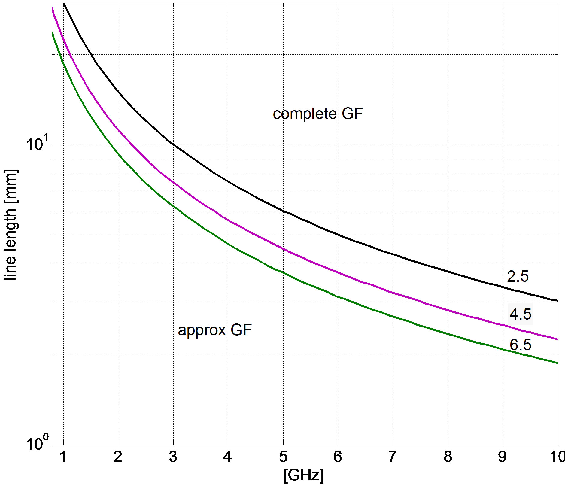 (b)
(b)
Figure 6. Regions for GFs evaluation for three permittivity values: (a) Dielectric thickness vs frequency; (b) Line length vs frequency.
reported in Table 1. Note that usually the dielectric thickness of the microstrips is much smaller than the limit values imposed by the map in Figure 6(a). This means that, usually, the main condition to check is that given in Figure 6(b), i.e. that on the trace length.
Let us first consider case C in Table 1. Figure 8 shows the absolute value of the current obtained by using
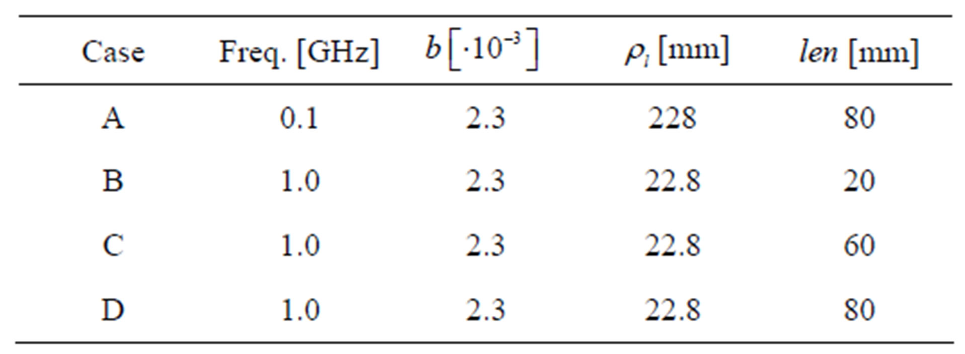
Table 1. Parameters for the considered cases.
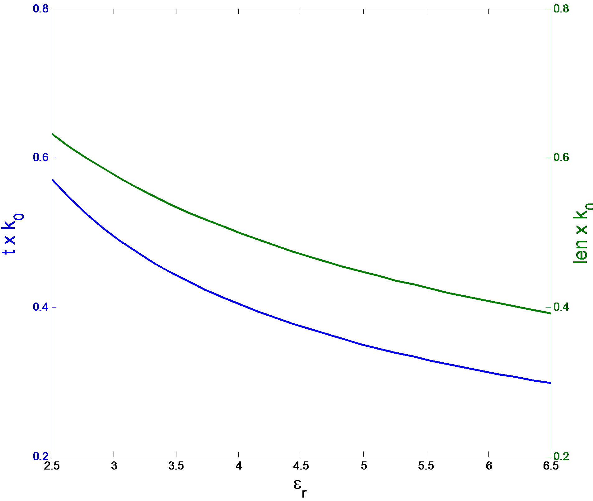
Figure 7. Regions for GFs evaluation: normalized dielectric thickness and line length, vs permittivity.
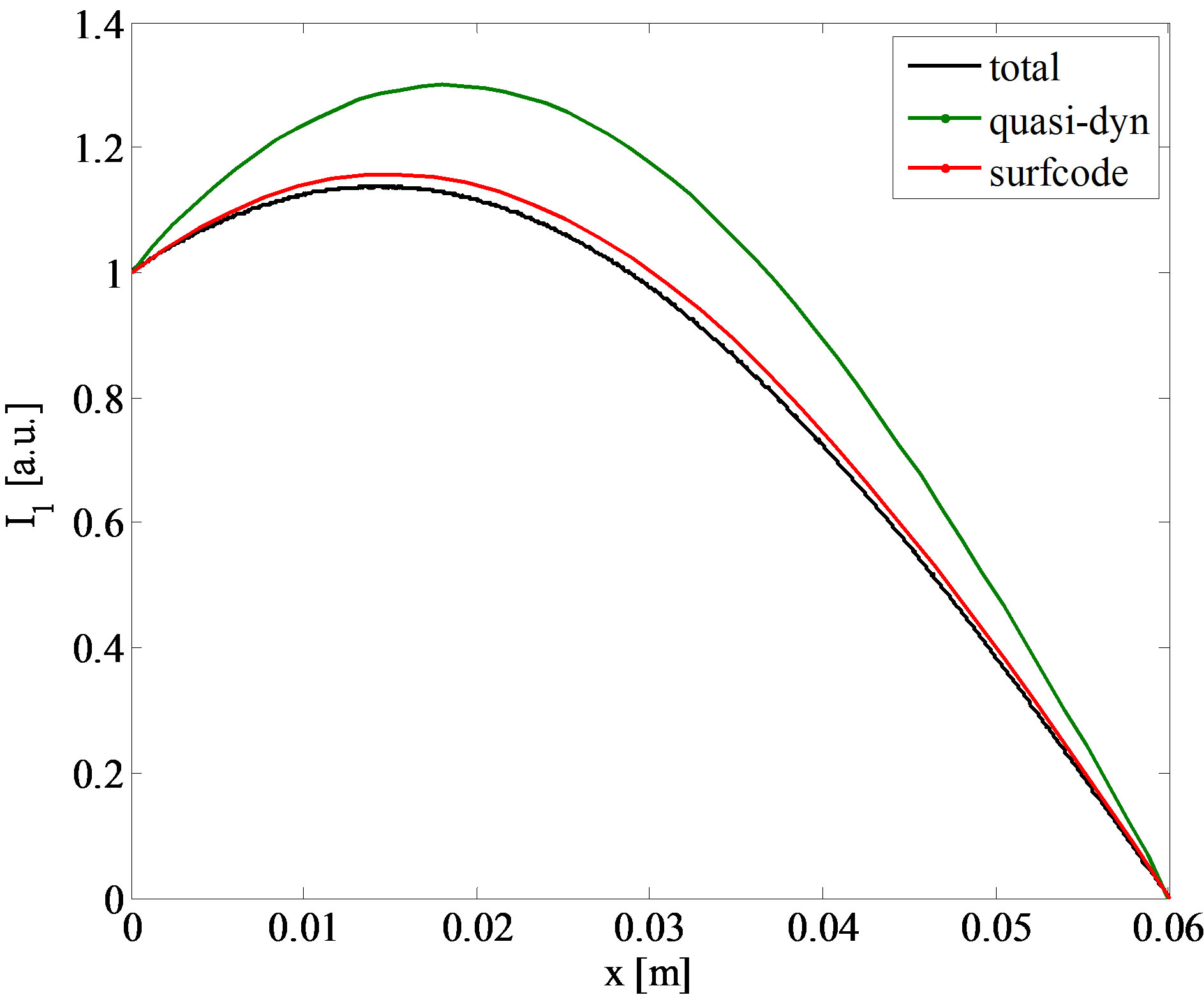
Figure 8. Absolute value of the spatial distribution of the current, case C.
 (a)
(a)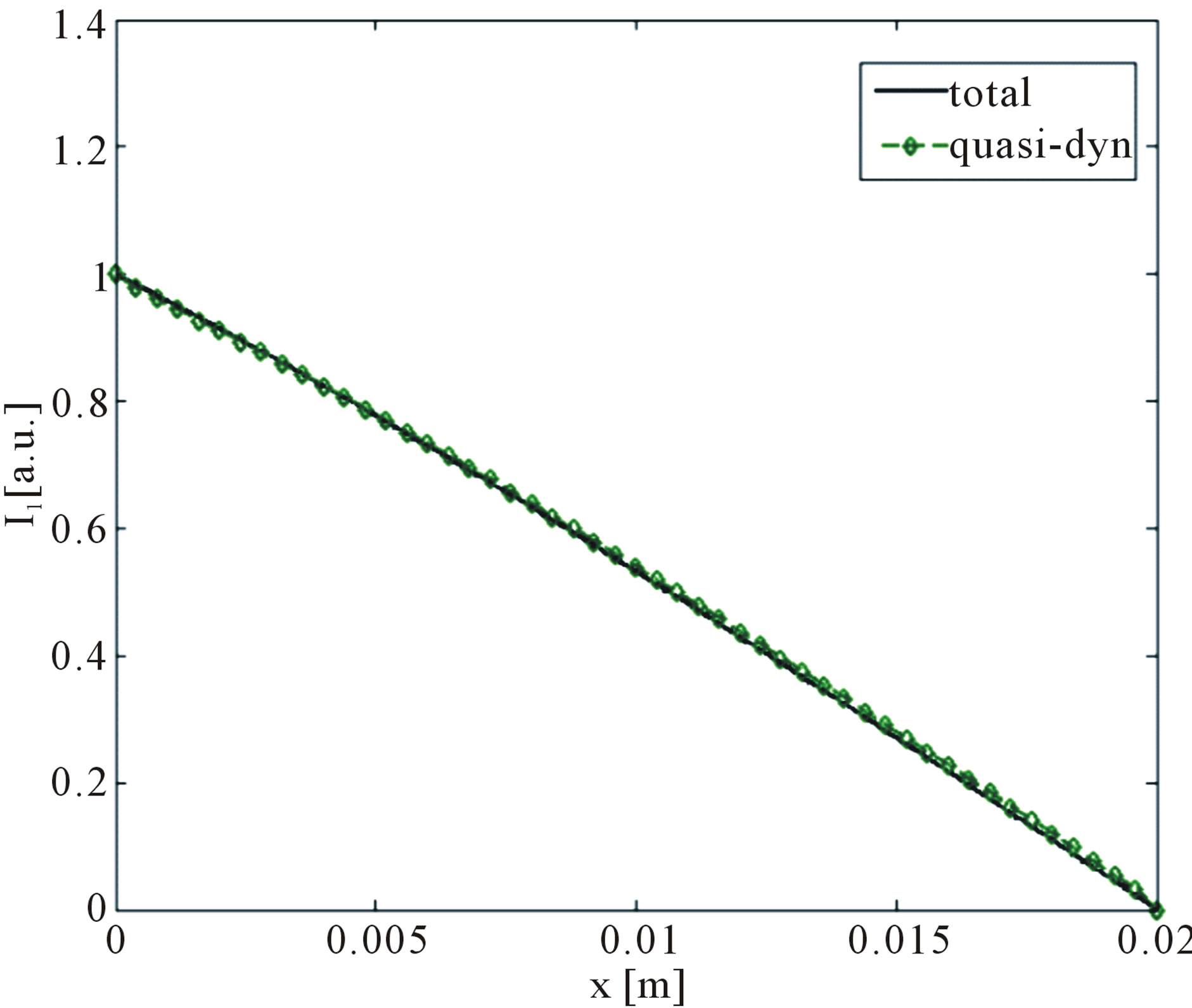 (b)
(b)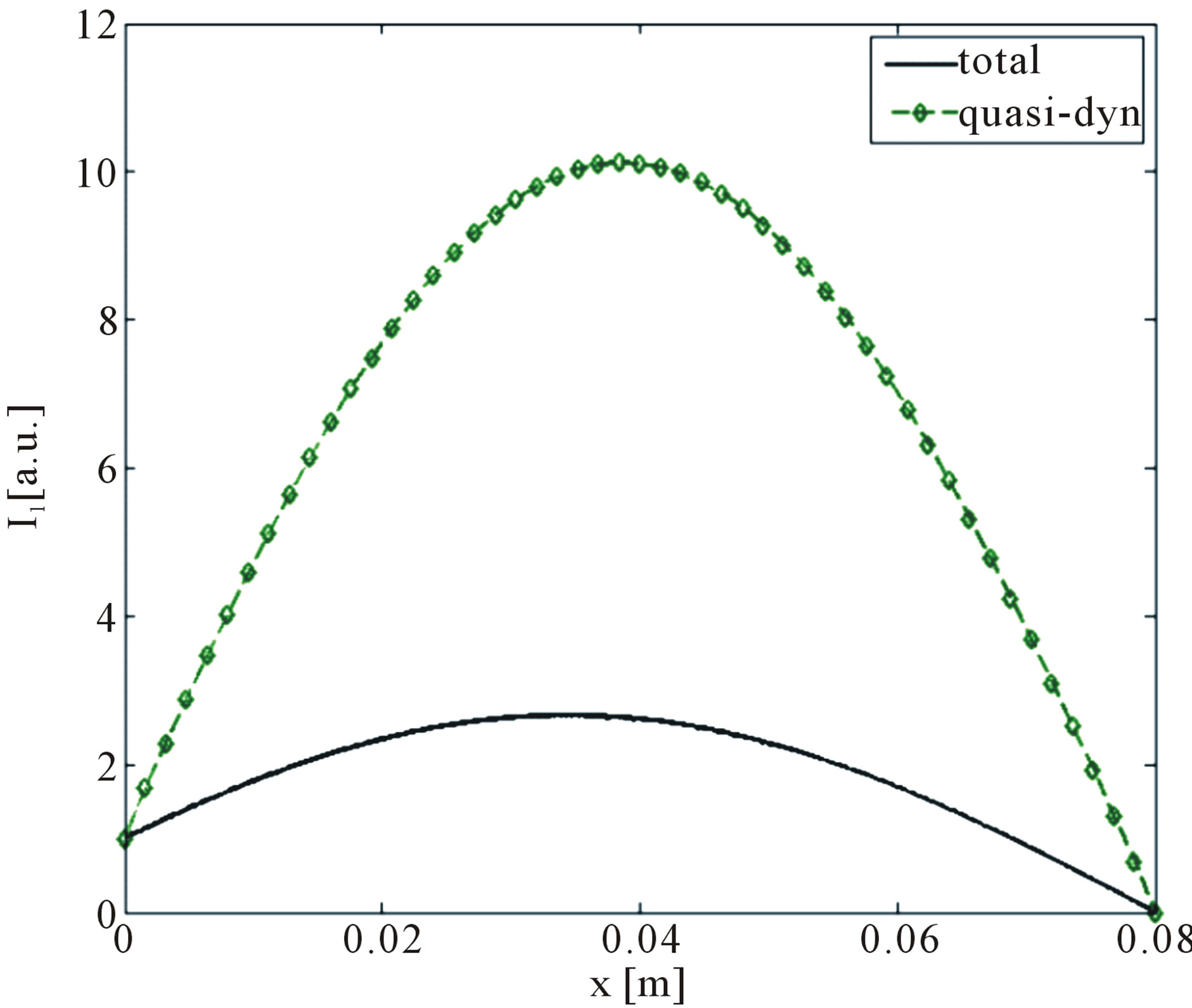 (c)
(c)
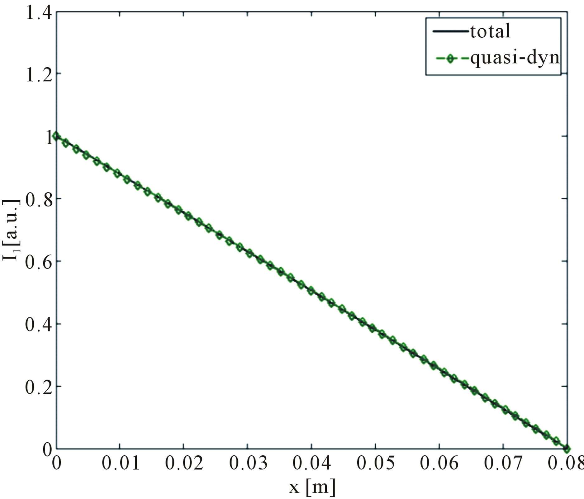
Figure 9. Absolute value of the spatial distribution of the current: (a) Case A; (b) Case B; (c) Case D.
the complete GF and the quasi-dynamic one. It is also reported the numerical solution provided by the fullwave 3D numerical SURFCODE [5], as a benchmark to assess the accuracy of the proposed model. For this case, the use of only the quasi-dynamic term would lead to inaccurate result, as clearly shown in Figure 8. This is consistent with the proposed criteria, since Case C does not fulfill the second of (26). Criteria (26) are satisfied in Case A and Case B but not in Case D. The results in Figures 9 confirm the reliability of such criteria.
5. Conclusions
In this paper, we have analyzed the problem of the efficient inclusion of layered media Green’s functions in electromagnetic integral formulations applied to the fullwave analysis of microstrips. Some of the most popular approximation techniques are briefly reviewed, all of them based on the decomposition of the spectral domain Green’s functions into a quasi-dynamic term and a dynamic one.
The spatial domain quasi-dynamic term may be found in closed form, which lowers the computational cost of the Sommerfeld integrals needed to inverse transform the Green’s functions from spectral to spatial domain. Therefore, it is of interest to assess some criteria to establish whether the quasi-dynamic terms approximate the complete Green’s functions.
A full-wave transmission line model has been used, implementing both the complete and the quasi-dynamic Green’s functions, and two simple conditions are proposed and verified. These conditions are written in terms of dielectric thickness, trace length, frequency and dielectric permittivity.
REFERENCES
- J. Mosig, “Arbitrarily Shaped Microstrip Structures and Their Analysis with a Mixed Potential Integral Equation,” IEEE Transactions on Microwave Theory and Techniaues, Vol. 36, No. 2, 1988, pp. 314-323. doi:10.1109/22.3520
- J. S. Zhao and W. C. Chew, “Integral Equation Solution of Maxwells Equations from Zero Frequency to Microwave Frequencies,” IEEE Transactions on Antennas and Propagation, Vol. 48, No. 10, 2000, pp. 1635-1645. doi:10.1109/8.899680
- R. F. Harrington, “Field Computation by Moment Methods,” IEEE Press, Piscataway, 1993.
- A. Ruehli, “Equivalent Circuit Models for Three-Dimensional Multiconductor Systems,” IEEE Transactions on Microwave Theory and Techniaues, Vol. 22, No. 3, 1974, pp. 216-221. doi:10.1109/TMTT.1974.1128204
- G. Miano and F. Villone, “A Surface Integral Formulation of Maxwell Equations for Topologically Complex Conducting Domains,” IEEE Transactions on Antennas and Propagation, Vol. 53, No. 12, 2005, pp. 4001-4014. doi:10.1109/TAP.2005.859898
- S. M. Holik and T. D. Drysdale, “Simplified Model of a Layer of Interconnects under a Spiral Inductor,” Journal of Electromagnetic Analysis and Applications, Vol. 3, No. 6, 2011, pp. 187-190. doi:10.4236/jemaa.2011.36031
- W. C. Chew, “Waves and Fields in Inhomogeneous Media,” IEEE Press, New York, 1995.
- C. A. Valagiannopoulos, “Semi-Analytic Solution to a Cylindrical Microstrip with Inhomogeneous Substrate,” Electromagnetics, Vol. 27, No. 8, 2007, pp. 527-544. doi:10.1080/02726340701669524
- Y. L. Chow, J. J. Yang, D. G. Fang and G. E. Howard, “A Closed-Form Spatial Green’s Function for the Thick Microstrip Substrate,” IEEE Transactions on Microwave Theory and Techniaues, Vol. 39, 1991, pp. 588-592. doi:10.1109/22.75309
- V. I. Okhmatovski and A. C. Cangellaris, “A New Technique for the Derivation of Closed-Form Electromagnetic Greens Functions for Unbounded Planar Layered Media”, IEEE Transactions on Antennas and Propagation, Vol. 54, No. 7, 2002, pp. 1005-1016. doi:10.1109/TAP.2002.800731
- M. I. Aksun and G. Dural, “Clarification of Issues on the Closed-Form Green’s Functions in Stratified Media,” IEEE Transactions on Antennas and Propagation, Vol. 53, No. 11, 2005, pp. 3644-3653. doi:10.1109/TAP.2005.858571
- V. N. Kourkoulos and A. C. Cangellaris, “Accurate Approximation of Green’s Functions in Planar Stratified Media in Terms of a finite Sum of Spherical and Cylindrical Waves,” IEEE Transactions on Antennas and Propagation, Vol. 54, No. 5, 2006, pp. 1568-1576. doi:10.1109/TAP.2006.874329
- E. Simsek, Q. H. Liu and B. Wei, “Singularity Subtraction for Evaluation of Green’s Functions for Multilayer Media,” IEEE Transactions on Microwave Theory and Techniaues, Vol. 54, No. 1, 2006, pp. 216-225. doi:10.1109/TMTT.2005.860304
- L. Feng, V. Okhmatovski, B. Song and A. Dengi, “Systematic Extraction of Static Images from Layered Media Green’s Function for Accurate DCIM Implementation,” Antennas and Wireless Propagation Letters, Vol. 6, No. 11, 2007, pp. 215-218.
- F. Mesa, R. R. Boix and F. Medina, “Closed-Form Expressions of Multilayered Planar Green’s Functions That Account for the Continuous Spectrum in the Far Field,” IEEE Transactions on Microwave Theory and Techniaues, Vol. 56, No. 7, 2008, pp. 1601-1614. doi:10.1109/TMTT.2008.925576
- M. Leone, “Design Expressions for the Trace-to-Edge Common-Mode Inductance of a Printed Circuit Board,” IEEE Transactions on Electromagnetic Compatibility, Vol. 43, No. 4, 2001, pp. 667-671. doi:10.1109/15.974648
- A. G. Chiariello, “New Models for High-Speed Interconnects: An Enhanced Transmission Line Model (ETL) for High-Speed Interconnects,” VDM Verlag, Berlin, 2009.
- A. G. Chiariello, A. Maffucci, G. Miano and F. Villone, “Transmission Line Models for High-Speed Conventional Interconnects and Metallic Carbon Nanotube Interconnects,” In: F. Rachidi and S. Tkachenko , Eds., Electromagnetic Field Interaction with Transmission Lines, WIT Press, Southampton, 2008. doi:10.2495/978-1-84564-063-7/06
- A. G. Chiariello, A. Maffucci, G. Miano, F. Villone and W. Zamboni, “A Transmission-Line Model for Full-Wave Analysis of Mixed-Mode Propagation,” IEEE Transactions on Advanced Packaging, Vol. 31, No. 2, 2008, pp. 275-284. doi:10.1109/TADVP.2008.920373
- A. G. Chiariello, G. Miano and A. Maffucci, “An Hybrid Model for the Evaluation of the Full-Wave Far-Field Radiated Emission from PCB Traces,” Progress in Electromagnetics Research, Vol. 101, 2010, pp.125-138. doi:10.2528/PIER09120905
- M. I. Aksun and R. Mittra, “Spurious Radiation from Microstrip Interconnects,” IEEE Transactions on Electron devices, Vol. 35, No. 2, 1993, pp. 148-158.
- K. A. Michalski and J. R. Mosig, “Multilayered Media Green’s Functions in Integral Equation Formulations,” IEEE Transactions on Antennas and Propagation, Vol. 45, No. 3, 1997, pp. 508-519. doi:10.1109/8.558666
NOTES
*Corresponding author.