Journal of Electromagnetic Analysis and Applications
Vol.4 No.3(2012), Article ID:18236,6 pages DOI:10.4236/jemaa.2012.43015
Optical Bistability in an Acousto-Optic Tunable Filter (AOTF) Operating with Short Optical Pulses
![]()
1Departamento de Física, Laboratório de Telecomunicações e Ciência e Engenharia de Materiais (LOCEM), Universidade Federal do Ceará, Fortaleza, Brazil; 2Faculdade de Educação de Crateús-Universidade Estadual do Ceará, Crateús, Brazil; 3Departamento de Teleinformática, Laboratório Especialista em Sistemas de Telecomunicações e Ensino (LESTE), Instituto Federal do Ceará (IFCE), Campus Fortaleza, Fortaleza, Brazil.
Email: *sombra@ufc.br
Received December 30th, 2011; revised February 5th, 2012; accepted February 15th, 2012
Keywords: Bistability; Acousto-Optic Tunable Filter
ABSTRACT
In this paper we report for the first time the presence of bistability in an acoustic-optic tunable filter (AOTF) operating with ultrashort (2 ps) optical light pulses. The results for the study of bistability has shown the dependence of the hysteresis curve with the product of the coupling constant (κ) by the length of the device (ξL) and the conversion power-coupling constant factor (G). The range of bistability varies significantly with both G and with kxL parameters. The variation of kxL directly increases the size of the range of bistability hysteresis while the increase in G causes the bistability to occur at low powers. The phenomenon of optical bistability (OB) is the object of increasing interest due to its possibilities for important device applications. A bistable device is a device with a capability to generate two different outputs for a given input and the physical requirements for this are an intensity-dependence refractive index and an optical feedback mechanism.
1. Introduction
The physical requirements for optical bistability (OB) are an intensity-dependence refractive index and an optical feedback mechanism [1]. A system is said to be optically bistable if it can exhibit two steady output states for the same input intensity over some range of input values. The switching up and down operations typical in a hysteresis cycle originates from the rise of instability. A physical state is said to be unstable when, after displaying the system a little from this steady point, the system does not return to it and goes further from it. In other words, for an unstable state, even the slightest perturbation removes the system from it. The searches for instabilities turn out to be crucial in the study of OB phenomena not only from the theoretical viewpoint but also for the possibilities for practical and technological applications.
Since its first discovery in late 1970’s, optical bistability has been found existing in many different optical systems. One of the simplest examples of bistable systems is a Fabry-Perot resonator with the cavity filled with a medium that presents saturable absorption or nonlinear dispersion. It has been established theoretically [2] and experimentally [3] that a Fabry-Perot interferometer filled with a nonlinear index medium exhibits bistability in response to optical inputs. Such a device has potential applications as an optical transistor, pulse shaper, memory element, and differential amplifier [4,5]. Generally, these optical systems fall into two categories: passive cavities containing either a saturable absorbing or a nonlinear dispersive medium, and laser systems with intracavity saturable absorbers [6,7]. The nonlinear effect of OB is currently under extensive investigation in a variety of different materials and systems [8]. This attention is justified mainly because the broad application of such systems in integrated optics and telecommunication.
The transmission of information by optical way has known a considerable progress which led the scientists to wonder about the possibilities of creating systems with purely optical memories. Actually due the increasing communications supply, it is necessary fast, reliable and chippers services. In this context it is natural the development of devices capable of processing ultrafast signals, so the importance of all-optical devices. The acousto-optic tunable filter (AOTF) is an example of this. The acoustooptic effect has been successfully used since the early 1980’s in the design and construction of a variety of optical fiber devices such as frequency shifters [9], tapers and couplers [10], filters [11,12] and modulators [13]. Particularly, acoustic waves can be employed to modulate the spectrum [14] and switch the wavelength [15] of fiber Bragg gratings. Specifically AOTF has attracted great attention in recent years, in part because it appears to be a suitable basis for multi-wavelength optical crossconnects [16]. Recent improvements in the AOTF design included passband engineering to reduce sidelobs [17], flatten the wavelength response [18], which reduce the crosstalk and increase the channel-width-to-channel-spacing ratio.
The AOTF is an all solid state electronic dispersive device which is based on the diffraction of light in a crystal [19-22]. Light is diffracted by an acoustic wave because when an acoustic wave propagates in a transparent material, it produces a periodic modulation of the index of refraction (via the elasto-optical effect). This, in turn, will create a moving grating which diffracts portions of an incident light beam. The diffraction process can, therefore, be considered as a transfer of energy and momentum [23].
2. Theoretical Framework
In our study we are considering the relative effects to the dispersion β(2) and nonlinearity γ coefficients over propagated pulses in the AOTF. The two-input ultrashort soliton pulses (2 ps) are polarized in the TE and TM modes. The amplitude of TE and TM modes are A1 and A2 respectively, as we can see in Equations (1) and (2). In this investigation, the input pulses have a hyperbolic form and the initial potency will vary intensity in a way we will describe more precisely afterwards. The temporal full width at halt maximum is ΔtPULSE = 2ln (1 + ) Δt0.
The coupled differential equations describing the evolution of the slowly varying complex modal field (A1 and A2) amplitudes of the pulse envelope in the AOTF [24,25] are:
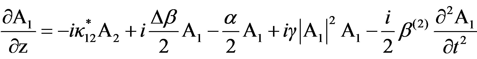 (1)
(1)
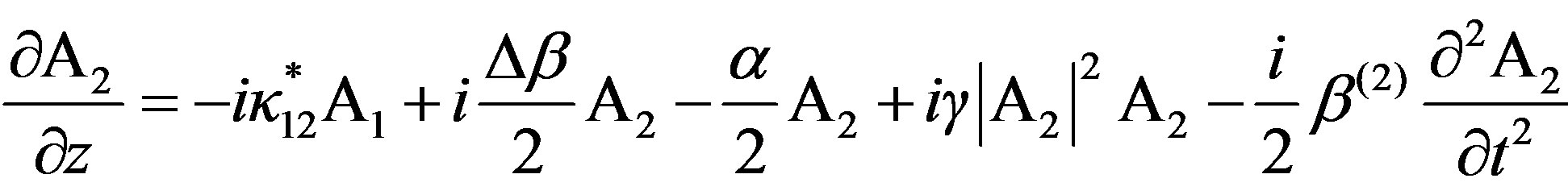 (2)
(2)
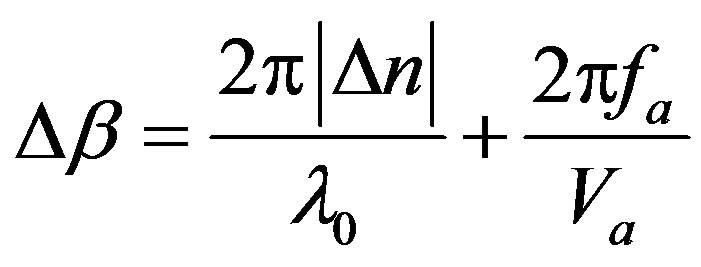
The Equation (1) is for the TE mode and the Equation (2) is for TM mode. The α parameter is the optical loss, κ12 is the linear coupling coefficient and Δβ = β1 – β2 ± K (β1 and β2 are the incident and diffracted light wave vectors components, respectively, along the direction of propagation of the acoustic wave with wave vector K is the momentum mismatch among the TE, TM modes and the acoustic wave). Further γ denotes the coefficient of self phase modulation (SPM), which is proportional to the nonlinear refractive index nNL of the material and β(2) represents the group-velocity dispersion parameter (GVD) of the optical medium. It is important to observer that in our study the sign of β(2) is negative so we have the anomalous propagation regime. In a collinear interaction the momentum mismatch of the modes is proportional to optical birefringence (Δn = n1 – n2) of the guide [25]:
 (3)
(3)
where λ0 is the pump wavelength, ƒa is the acoustic frequency and Va is the velocity of sound in the optical medium. When the phase-matching condition (Bragg condition) is satisfied (Δβ = 0), one knows the acoustic frequency necessary for exact tuning of the pump wavelength λ0. We will suppose an ideal AOTF normally operating at the condition when |κ12|ξL = π/2 (ξL is the acousto-optic interaction length). So the power conversion is 100% (maximum efficiency in the conversion of energy among the coupled modes) when the phasematching condition is satisfied. Consequently, for a collinear interaction, the full bandwidth at half maximum of the AOTF (Δƒaotf) is inversely proportional to birefringence (Δn) and acoustic-optical interaction length (ξL) through of relation:
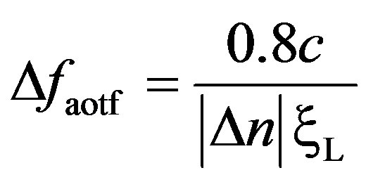 (4)
(4)
where c is velocity of light in the vacuum.
The manufacturing process of AOTF and the physical consequences of the choice of the material used to its construction can be found elsewhere [26-29]. In our study we are considering a centro-symmetric material, as the germanium crystal (Ge), to avoid the presence of the effects of second-order [χ(2)] nonlinear susceptibility. For this choice, the principal refraction indexes could be found in [23].
3. Numerical Procedure
To study OB one need to choose just one polarization in the output of the device and that same polarization will receive the feedback. Here the polarization that is studied is TE. The proposed model for the investigation of the performance of the AOTF as a bistable device possesses the architecture shown in the Figure 1. It consists of an optical waveguide occupying the same space as an acoustic waveguide. The acoustic wave is introduced into the acoustic guide using a surface acoustic wave (SAW) transducer. The acoustic field acts on the optical fields in the interaction region to convert the TE polarization to a TM mode, and vice versa. This interaction is frequency selective because of the requirement for momentum matching for significant interaction. The polarization conversion efficiency can be calculated by treating the

Figure 1. Schematic of the acousto-optic tunable filter device with the feedback structure for the output of TE mode.
device as a classical directional coupler, where the coupled modes are the TE and TM modes of the optical waveguide, and the coupling coefficient is proportional to the acoustic amplitude.
The TE and TM input modes go throughout the AOTF. After this the pulses pass in a polarization beam splitter where a small part of the TE transmitted beam is monitored by a photodiode detector whose output is proportional to the transmitted light intensity. Such beam is then amplified and the signal will pump the RF signal to be used as feedback to feeds the transducer. The proposed feedback can vary the acoustic wave intensity of frequency. It is possible to consider these effects separately. The radiofrequency amplitude, RF, controls the variation of the transmitted light intensity. This is equivalent to vary the product kxL in the optic domain. However, the RF signal controls the acoustic-optic frequency and determines the optic frequency or wavelength. Figure 2 shows the polarization conversion efficiency between the modes with the change in .
.
Considering the proposed feedback, the change in the phase matching will be analyzed and interpreted by the following expression:
 (5)
(5)
Here,  is the initial phase matching (without feedback). Figure 2 shows how the intensity modifies when the
  value changes. We suppose here the effect of the feedback is to change the
  value and the G parameter controls that changing. The P0S factor is associated to the fact that the change is proportional to the feedback intensity. The G parameter represents how much of the TE feedback will be used by the transducer to modify the acoustic wave inside the device. It is important to notice that this feedback structure will be responsible for the bistable response.
In Equations (1) and (2) the time t = t' – z/υg is measured in a frame of reference moving with the pulse in the group-velocity (υg). We have analyzed numerically the ultrashort pulse transmission in the anomalous propagation
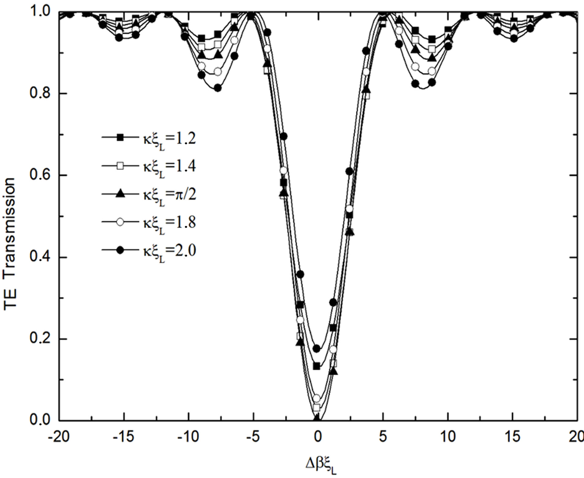
Figure 2. Transmission curves for output TE mode.
regime through the AOTF. We are considering that the full temporal width at half maximum of the input pulses is Δtpulse = 2 ps, corresponding to a full spectral bandwidth at half maximum Δƒpulse = 0.157 THz. The general form of the initials pulses at the AOTF input is given by:
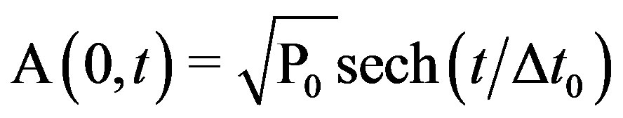 (6)
(6)
The power for TE mode will suffer two process; in the first it will vary from 0 W to 30 W, and after this it will vary from 30 W to 0 W. For ultrashort soliton pulses of Δtpulse = 2 ps, one has Δt0 = 1.135 ps. The AOTF length used was approximately ξL = 21.8 mm using the parameterized value Δn = 0.07 for the induced birefringence in the material. Starting this point one calculates the dispersive e nonlinear coefficients β(2) = –0.127 ´ 10–27 ps2/mm and γ = 0.098 ´ 10–3 (w·mm)–1, respectively, for the numeric study of the proposed model.
The system of coupled NLS Equations (1) and (2) was solved numerically using the 4th order Runge-Kutta method with 1024 temporal grid points taking in account the initial conditions given by Equation (6), in the situation without loss (α = 0). In order to solve the system of coupled NLSE with this method, used only to ordinary differential equations, was necessary replace the differential operator  by –ω2, where ω is the frequency in the Fourier domain. Since ω is just a number in Fourier space, the use of the FFT algorithm makes numerical evaluation of the last terms on the right side of (1) e (2) straightforward and relatively fast [30]. Many of the features of the diffraction of light by sound can be deduced if we take advantage of the dual particle-wave nature of light and of sound. The diffraction of light by sound can be described as a sum of single collisions, each of which involves the annihilation of one incident photon at ω1 and one phonon at Ω and simultaneous creation of a new (diffracted) photon at a frequency ω2 = ω1 ± Ω. Thus the converted light between the two modes is shifted in frequency by an amount equal to the sound frequency. Since the sound frequencies of interest are below 1010 Hz and those of the incident light are usually above 1013 Hz, one has that ω2 ≈ ω1 = ω = 2πc/λ0 . This simplifies the computational numeric study of the Equations (1) and (2).
In our present configuration of study, we will use in the TM input (see Figure 1), a mode-locking laser with 2 ps of pulse duration and a repetition rate necessary to have the TE output to be in phase with the next pulse of the TM train in the input of the device. This is necessary to guarantee the feedback in the operation of the device. Considering for example that for a device of 21.8 mm, we will have a delay around 70 ps for the feedback signal to interact with the next pulse of the train in the TM input. In this case our system has to operate at a repetition rate around 14 GHz to maintain this sincronization.
4. Results and Discussions
In Figure 3, we could initially appreciate a hysteresis curve achieved when the parameters kxL = 1.2 and G = 100. The abscissa axis (Ii) represents the input power intensity at the AOTF and the ordinate axis (Io) represents the output power intensity. The trajectory indicated by Up represents TE power increasing and the trajectory indicated by Down represents the case for TE power decreasing. A little analysis could be outlined to describe the phenomenon. For conditions in with the transmitted intensity increases faster than the incident intensity, the nonlinear response of the device can be used for differential gain in a manner similar to transistor amplifiers. In this situation, a small modulation on the incident light wave can be converted to a larger modulation on the transmitted wave.
It is also possible to observe in the same figure the range of the OB for the parameters chosen it is something about 20 - 22.4 W for input power intensity. Figure 4 shows us that a change in just one of these parameters will vary this range. The value used for gain was G = 300 when we varied the kxL values. For kxL = 1.2, representing here by the solid line, the optical bistability range varies something about 6.4 - 7.6 W. Another curve represents the curve for kxL = 1.4 as indicated in the figure. It now possible to compare the effect on the optical bistability range; the range for kxL = 1.4 is something about 6.5 - 12.2 W; almost five times bigger.
Figure 4 shows the optical bistability behavior analysis when the kxL value is sustained and G values varies. For this analysis we chose kxL = 1.2 and the values for G are indicated in the figure. The first thing we could note is that with increasing the G value the critical powers of the hysteresis curve are decreasing. Another important fact to note is that when the increasing of G the hysteresis curve tends to decrease the internal area of the hysteresis
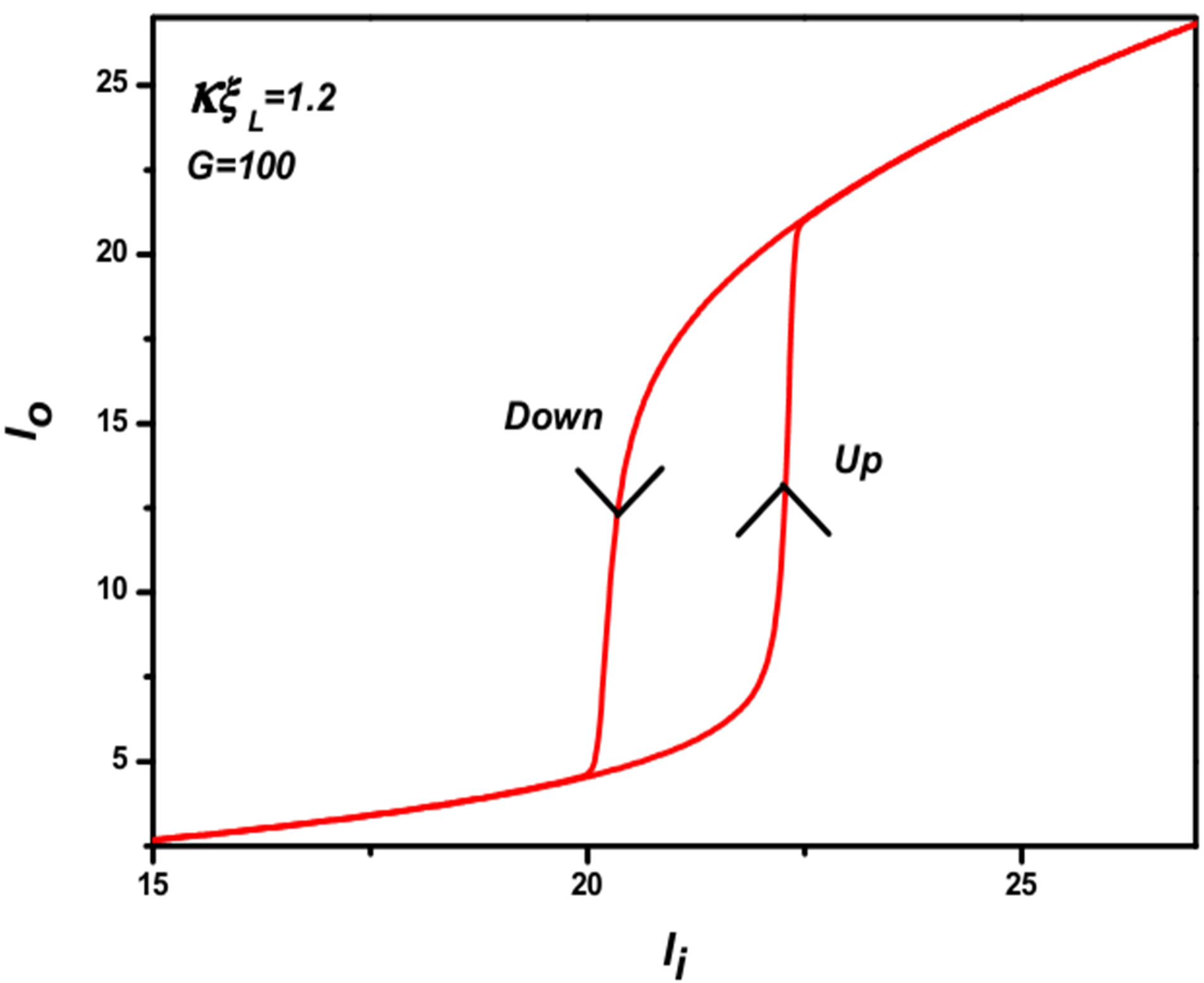
Figure 3. Hysteresis curve for parameters kxL = 1.2 and G = 100. Ii is the input power intensity at the AOTF and the Io the output power intensity. Up represents the trajectory for G(P) positive and Down for G(P) negative.
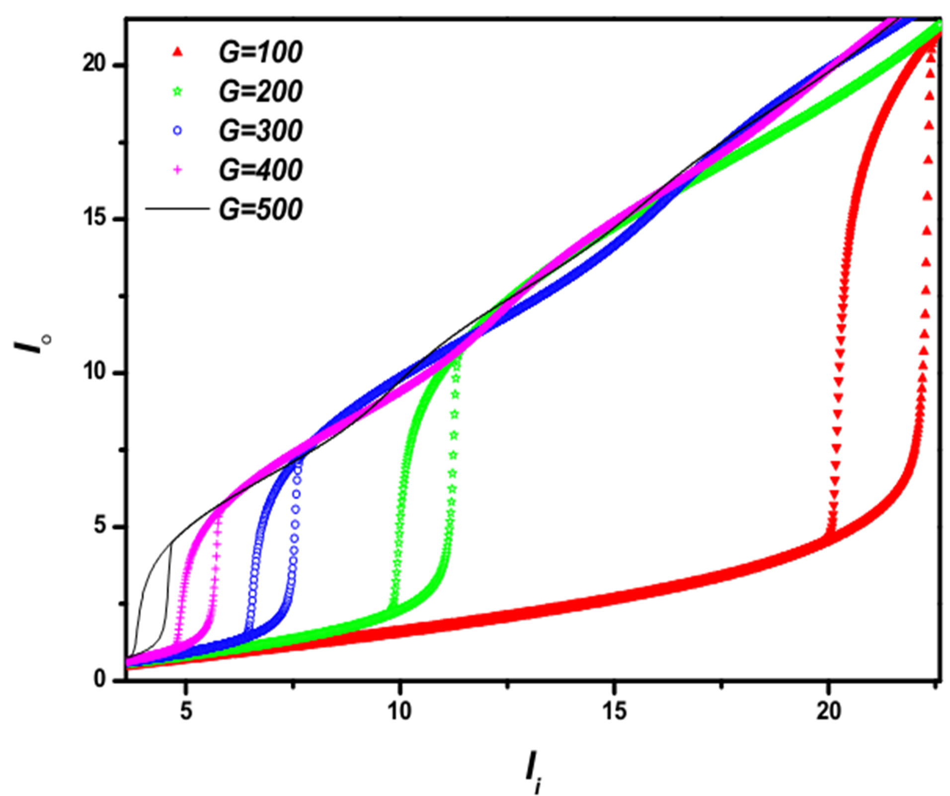
Figure 4. Hysteresis curves for kxL = 1.2 and G varying.
curve. This great difference for example between G = 100 and G = 200 would be very important in practical applications.
Figure 2 should help us to understand what kind of process is occurring. One can see that the energy transmission is inversely proportional to the coupling constant factor. That agree with the Equations (1) and (2), since the first term of the right side in those equations is increasing and the coupling is making stronger. Less energy is left for the TE mode when the coupling increases; so the critical power of the hysteresis curve is increasing. In other words, the system will take a long time to saturate.
When the change occurs in the G parameter, the second term of the right side of Equations (1) and (2) are increasing this time. The coupling is not getting stronger and the energy transmission to another mode is smaller when G increases. The Figure 5 shows us that the effect of this will be the difference of output energy intensity for a little change in the input energy intensity.
5. Conclusions
In this paper we report for the first time the presence of bistability in an acoustic-optic tunable filter (AOTF) operating with ultrashort (2 ps) optical light pulses. The results for the study of bistability has shown the dependence of the hysteresis curve with the product of the coupling constant (κ) by the length of the device (xL) and the conversion power-coupling constant factor (G). The range of bistability varies significantly with both G and with kxL parameters. The variation of kxL directly increases the size of the range of bistability hysteresis while the increase in G causes the bistability to occur at low powers. A bistable device is a device with a capability to generate two different outputs for a given input and the physical requirements for this are an intensity-dependence refractive index and an optical feedback mechanism.
A possible mechanism for this is behavior is a strong dependence of the optical intensity on the index of refraction as defined as a feedback function in the TE mode. The optical bistability has been used in a great range of applications like optical transistor, element, differential amplifier, etc. In this work we vary basically two kinds of parameters. We observe that the kxL and G parameters will control the bistable behavior of the device.
The phenomenon of optical bistability (OB) is the object of increasing interest due to its possibilities for important device applications.
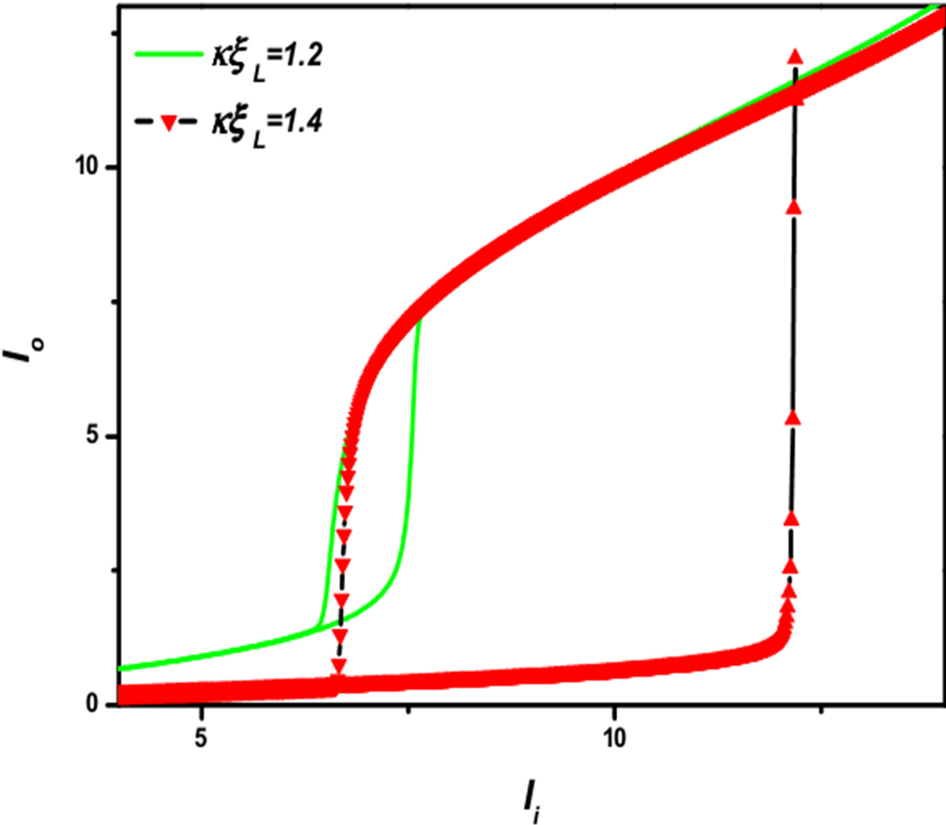
Figure 5. Hysteresis curves for G = 300 comparing the bistability ranges between kxL = 1.2 and kxL = 1.4.
6. Acknowledgements
We thank CAPES (Coordenação de Aperfeiçoamento de Pessoal de Nível Superior), CNPq (Conselho Nacional de Desenvolvimento Científico e Tecnológico), FINEP (Financiadora de Estudos e Projetos), FUNCAP (Fundação Cearense de Amparo a Pesquisa) for the financial support and CENTEC (Instituto Centro de Ensino Tecnológico).
REFERENCES
- R. Stofferl and Y. S. Kivshar, “Optical Bistability in a Nonlinear Photonic Crystal Waveguide Notch Filter,” Proceedings Symposium IEEE/LEOS Benelux Chapter, Delft, 2000, pp. 247-250.
- F. S. Felber and J. H. Marburger, “Theory of Nonresonant Multistable Optical Devices,” Applied Physics Letters, Vol. 28, No. 731, 1976, pp. 335-342. doi:10.1063/1.88632
- J. H. Marburger and F. S. Felber, “Theory of a Lossless Nonlinear Fabry-Perot Interferometer,” Physical Review A, Vol. 17, 1978, pp. 335-342. doi:10.1103/PhysRevA.17.335
- H. G. Winful, J. H. Marburger and E. Garmire, “Theory of Bistability in Nonlinear Distributed Feedback Structures,” Applied Physics Letters, Vol. 35, No. 5, 1979, p. 379. doi:10.1063/1.91131
- P. W. Hawkes, “Advances in Electronics and Electron Physcs,” Academic Press, Inc., London, 1994.
- A. E. Siegman, “Lasers,” University Science Books, Mill Valley, 1986.
- R. W. Boyd, “Nonlinear Optics,” Academic Press, Inc., San Diego, 1992.
- C. Bowden, M. Ciftan and H. R. Robl, “Optical Bistability,” Plenum, New York, 1981. doi:10.1007/978-1-4684-3941-0
- B. Y. Kim, J. N. Blake, H. E. Engan and H. J. Shaw, “AllFiber Acousto-Optic Frequency Shifter,” Optics Letters, Vol. 11, No. 6, 1986, pp. 389-391. doi:10.1364/OL.11.000389
- T. A. Birks, P. St. J. Russel and D. O. Culverhouse, “The Acoust-Optic Effectin Single-Mode Fiber Tapers and Couplers,” Journal of Lightwave Technology, Vol. 14, No. 11, 1996, pp. 2519-2529. doi:10.1109/50.548150
- R. Feced, C. Alegria, M. N. Zervas and R. I. Laming, “Acoustooptic Attenuation Filters Based on Tapered Optical Fibers,” IEEE Journal of Selected Topics in Quantum Electronics, Vol. 5, No. 5, 1999, pp. 1278-1288. doi:10.1109/2944.806753
- A. Díez, M. Delgado-Pinar, J. Mora, J. L. Cruz and M. V. Andrés, “Dynamic Fiber-Optic Add-drop Multiplexer Using Bragg Gratings and Acousto-Optic-Induced Coupling,” Technology Letters, Vol. 15, No. 1, 2003, pp. 84-86. doi:10.1109/LPT.2002.805867
- R. A. Oliveira, C. A. F. Marques, C. E. N. Mayer, J. T. Pereira, R. N. Nogueira and A. A. P. Pohl, “Single Device for Excitation of Both Flexural and Longitudinal AcoustoOptic Effects in Fiber Bragg Gratings,” Microwave and Optoelectronics International Conference (IMOC), 2009 SBMO/IEEE MTT-S, Belem, 3-6 November 2009, pp. 546-549. doi:10.1109/IMOC.2009.5427526
- W. F. Liu, P. St. J. Russell and L. Dong, “Acousto-Optic Superlattice Modulator Using a Fiber Bragg Grating,” Optics Letters, Vol. 22, No. 19, 1997, pp. 1515-1517. doi:10.1364/OL.22.001515
- W.-F. Liu, I-M. Liu, L.-W. Chung, D.-W. Huang and C. C. Yang, “Acoustic-Induced Switching of the Reflection Wavelength in a Fiber Bragg Grating,” Optics Letters, Vol. 25, No. 18, 2000, pp. 1319-1321. doi:10.1364/OL.25.001319
- B. L. Heffner, D. A Smith, J. E. Baran and K. W. Cheung, “Integrated Optic Acoustically-Tunable Infrared Optical Filter,” Electronics Letters, Vol. 24, No. 1, 1988, pp. 1562- 1563. doi:10.1049/el:19881065
- H. Hermann and St. Schmidt, “Integrated Acousto-Optical Mode Converters with Weighted Coupling Using Surface Acoustic Wave Directional Couplers,” Electronics Letters, Vol. 28, No. 11, 1992, pp. 979-980. doi:10.1049/el:19920622
- D. A. Smith, J. E. Baran, J. J. Johnson and K.-W. Cheung, “Integrated-Optic Acoustically Tunable Filters for WDM Networks,” IEEE Journal on Selected Areas in Communication, Vol. 8, No. 6, 1990, pp. 1151-1159.
- C. D. Tran and R. J. Furlan, “Spectrofluorometer Based on Acousto-Optic Tunable Filters for Rapid Scanning and Multicomponent Sample Analyses,” Analytical Chemistry, Vol. 65, No. 13, 1993, pp. 1675-1681. doi:10.1021/ac00061a008
- D. Chieu and L. Jian, “Characterization of the AcoustoOptic Tunable Filter for the Ultraviolet and Visible Regions and Development of an Acousto-Optic Tunable Filter Based Rapid Scanning Detector for High-Performance Liquid Chromatography,” Analytical Chimica Acta, Vol. 314, No. 57, 1995, pp. 57-66. doi:10.1016/0003-2670(95)00306
- C. D. Tran and G. H. Gao, “Characterization of an Erbium-Doped Fiber Amplifier as a Light Source and Development of a Near-Infrared Spectrophotometer Based on the EDFA and an Acoustooptic Tunable Filter,” Analytical Chemistry, Vol. 68, No. 13, 1996, pp. 2264-2269. doi:10.1021/ac9600262
- C. Pasquini, J. Lu, C. D. Tran and S. Smirnov, “Detection of Flow Injection Analysis with Ph Gradient by AcoustoOptic Tunable Filter Based Spectrophotometry,” Analytica Chimica Acta, Vol. 319, No. 3, 1996, pp. 315-324. doi:10.1016/0003-2670(95)00509-9
- A. Yariv and P. Yeh, “Optical Waves in Crystal: Propagation and Control of Laser Adiation,” John Wiley and Sons, New York, 1984.
- C. S. Sobrinho and A. S. B. Sombra. “Picosecond Pulse Switching in an Acousto-Optic Tunable Filter (AOTF) with Loss,” Nonlinear Optics, Vol. 29. No. 1, 2002, pp. 79-97. doi:10.1080/10587260213929
- C. S. Sobrinho, J. L. S. Lima, E. F. de Almeida and A. S. B. Sombra, “Acousto-Optic Tunable Filter (AOTF) with Increasing Non-Linearity and Loss,” Optics Communications, Vol. 208, No. 4, 2002, pp. 415-426. doi:10.1016/S0030-4018(02)01599-7
- C. D. Tran, “Principles and Analytical Applications of Acousto-Optic Tunable Filters, an Overview,” Talanta, Vol. 45, No. 2, 1997, pp. 237-248. doi:10.1016/S0039-9140(97)00146
- Y. Jung, S. B. Lee, J. W. Lee and K. Oh, “Bandwidth Control in a Hybrid Fiber Acousto-Optic Filter,” Optics Letters, Vol. 30, No. 1, 2005, pp. 84-86. doi:10.1364/OL.30.000084
- C. S. Sobrinho, A. F. G. F. Filho, J. C. Sales, A. F. M. Neto, E. F. de Almeida and A. S. B. Sombra, “AcoustoOptic Tunable Filter (AOTF) Revisited: Ultrashort Optical Pulses Crosstalk Studies on the Lossy Filter,” Fiber and Integrated Optics, Vol. 25, No. 3, 2006, pp. 195-211. doi:10.1080/01468030600569834
- C. S. Sobrinho, C. S. N. Rios and A. S. B. Sombra, “Integrated Acousto-Optical Temperature Sensor,” Fiber and Integrated Optics, Vol. 25, No. 6, 2006, pp. 387-402. doi:10.1080/01468030600910731
- T. R. Taha and M. J. Ablowitz, “Analytical and Numerical Aspects of Certain Nonlinear Evolution Equations. II. Numerical, Nonlinear Schrödinger Equation,” Journal of Computational Physics, Vol. 55, No. 2, 1984, pp. 203- 230. doi:10.1016/0021-9991(84)90003-2
NOTES
*Corresponding author.