Journal of Electromagnetic Analysis and Applications
Vol. 2 No. 3 (2010) , Article ID: 1539 , 6 pages DOI:10.4236/jemaa.2010.23020
Modeling of the Earth’s Planetary Heat Balance with Electrical Circuit Analogy
![]()
Pulkovo Observatory, St. Petersburg, Russia.
Email: abduss@gao.spb.ru
Received December 4th, 2009; revised January 12th, 2010; accepted January 17th, 2010.
Keywords: Electrical Circuit Analogy, Planetary Heat Balance, Climate Trends
ABSTRACT
The integral heat model for the system of the Earth’s surface—the atmosphere—the open space based on the electrical circuit analogy is presented. Mathematical models of the heat balance for this system are proposed. Heat circuit which is analog of the electrical circuit for investigating the temperature dependencies on the key parameters in the clear form is presented.
1. Introduction
Electrical circuit analogy can be effectively used in termophysical applications [1]. Ohm’s and Kirchhoff’s laws are work in equivalent schemes with lumped parameters; heat fluxes are analogues of currents, heat conductivity (or heat resistance) is analog of the electrical resistance, and temperatures are analogues of the electrical potential. The purpose of this work is to use this method for development of the integral analytical model of the heat balance based on the equivalence scheme for the system the surface—the atmosphere—the open space describing heat processes clearly.
Variations of surface and atmospheric radiative parameters and atmospheric transparency for the surface radiation have important influence on the Earth’s climate. The simplest and convincing explanation of calculated dependencies is obtained with conversion from radiative characteristics to specific heat conductivities.
In this work we have restricted with analysis of how atmospheric transparency for the heat IR radiation from the surface influences on the climate. It is a topical problem, because nowadays this transparency is regarded as one of the cardinal factors making the climate. To reach the general result, we are investigated all range of the possible transparency changed from 0 to 1.
2. Physical Model
Method of the electrical circuit analogy can be used for a system of isothermal bodies having small heterogeneities, its make it possible to establish connection among schematic nodes with heat conductivities, and nodes define temperatures. In other words, the electrical circuit analogy can be used for the heat exchange problem and can’t be used for the heat conduction problem. So we regard the atmosphere as the homogeneous cover for the surface. The assumption is adopted that all atmospheric heterogeneities on the vertical dimension (pressure, density, temperature profiles) don’t influence on heat conditions of the underlying surface. We operate the surface temperature averaged on the whole surface (including the land and the ocean) and the atmospheric temperature averaged on the atmospheric volume.
These simplifications are brought to the idealized model of the system which contains the isothermal spherical core inside the isothermal spherical cover. The heat sources caused by the incoming solar radiation acts on the cover surface and in the cover (in W/m2). These heat sources are uniformly distributed.
In generally accepted practice the absorbed heat fluxes averaged and uniformly distributed on all the spherical surface are used [2]. It is reasonable by the Earth’s rotation around terrestrial axis, and assumption is adopted that speed of this rotation is greater than warming or cooling rate (in days-1). In other words, the Earth’s orbital period is considerably smaller than the value of the thermal inertia. This fact justifies using of averaged atmospheric and surface temperatures as criteria of the climate state. The core and the cover are in the convective and radiative heat exchange with each other. The cover is partially transparent for the core heat radiation and also gives the heat energy with the radiation to the open space itself.
The developed equivalent scheme is shown in Figure 1 Three levels are notable: the first level corresponds to the surface with the highest temperature Тs, the second level corresponds to the atmospheric averaged on volume temperature Та, and the third one corresponds to the open space temperature Тe assumed equals to zero, Тe = 0K. The biggest part of the surface is the ocean, so we use the heat capacity of the ocean describing transient behavior.
Heat sources Qs and Qa are analogues of current sources: Qs—specific power of the heat emission on the surfaces of the land and the ocean; Qa—specific power of the heat emission in the atmosphere. Sources of the temperature force, which are analogues of voltage, are omitted on the scheme as temperatures Тs and Та are potentials depending on scheme parameters. Surface capacities of the ocean and the atmosphere Сs and Са in J/m2K are analogues of the electrical capacity. Nodes are connected with conductivities, through its specific heat fluxes qi are flowing. Radiative conductivities αs, αa, αr presents as electrical resistance usually presents. The black frame denotes the specific heat conductivity α, which is resultant total convective and evaporating-condensation coefficient of the heat transfer from the ocean surface to the atmosphere in W/m2K.
Flux qs is a radiative flux transferred from the ocean surface to the open space directly through atmospheric window. Specific flux qа is defining power of the heat radiation from the atmosphere to the open space, and qr is the resultant radiative flux between the ocean and the atmosphere and it describes difference between fluxes transferred with the radiation from the ocean surface to the atmosphere and from the atmosphere to the ocean. Specific heat flux q is a resultant flux transferred by the convection and evaporating-condensation mechanism from the ocean to the atmosphere.
In the transient heat state the change of the heat con-
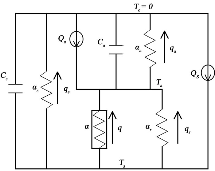
Figure 1. The equivalent thermal scheme based on the electrical circuit analogy corresponds to the model of planetary heat balance. Arrows shows the directions of the heat fluxes q. Q are sources of heat power. C are capacities. α are conductivities. See in text the detailed description of the scheme elements
tent in the atmosphere and the ocean mixed layer is taking into account with the flux from the capacities Cs and Ca. The isothermal active layer can be allocated for the ocean with the layer thickness lo, it depth depends on the convective hashing of water in it. For the land it is necessary to take into account unevenness of temperature distribution in the soil thickness, it is attained with using the transient heat equation. On this stage we don’t consider this problem, because the electrical circuit analogy can’t be used to solve it.
Integral emissivities and basic values of atmospheric transmission in IR range are used to define coefficient of radiative heat transfer and heat fluxes. For specificity it is necessary to introduce some assumptions about its:
• surface emissivity is obtained as averaged on the whole ocean and land, it averaged value is defined from conditions of the heat balance;
• averaged values of atmospheric emissivity with regard to averaged cloudiness is obtained the same in the direction to the space and in the direction to the surface;
• radiative balance is described using net heat flux and transfer factor, last one is deduced through wellknown way [1];
• atmospheric transmission for IR spectral range taking into account with it averaged values for atmospheric windows (main atmospheric window is the range 8.13 µm) [3].
There are two main reasons to use this model to analysis of the climatic global trends.
First, the ocean is the main part of the surface (more then 75% of it). The ocean has a very big thermal inertia caused by its very big thermal capacity. As it shown below, the constant of thermal inertia is about 8.5 years or more. As result, the surface temperature doesn’t change seriously during one day for both lighted and shadowed parts of the surface. That’s why the averaged temperature of surface can be used. This fact presents on the scheme with node having temperature Ts.
The values of the atmospheric density and the atmospheric capacity are an additional factor to the first one described above. Both factors make it valid and efficient to investigate the global climatic trends with the model based on the equivalent thermal scheme, which is build with electrical circuit analogy.
3. Mathematical Model
For composing the heat balance of the system of the surface—the atmosphere, the general equation system describing the heat exchange among isothermal bodies is introduced [1]. In the most general case the heat exchange among n bodies is described by the ordinary differential equation system, which contains n equations [1]
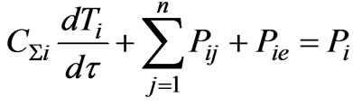 (1)
(1)
Initial conditions are usually setting in form
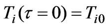 (2)
(2)
In our case it is convenient to use the specific heat fluxes qij, qie and Qi defined by rates qij = Pij/Si, qie = Pie/Si, Qi = Pi/Si; here Si – surface area of body no. i taking part in heat exchange. As result, the equations from the system (1) are expressed as
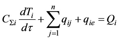 (3)
(3)
Surface dencities of total capacities Ci are defined from rates Ci = CΣi/Si.
Specific heat fluxes can be setting in form
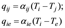 (4)
(4)
Here αij and αie—conductivities for heat transfer from body no. i to body no. j and from body no. i to environment, respectively; Ti, Tj and Te—absolute temperature of bodies i, j and environment.
In the beginning we use the simplified steady-state situation corresponded to the mathematical description (3) of the scheme in Figure 1.
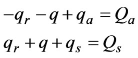 (5)
(5)
Fluxes in the system (5) are defined from rates
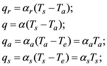 (6)
(6)
This system (5) contains the four unknowns (qr, q, qa, qs) and two equations, so it can’t be solved unequivocally. However, for the heat circuit the problem is simplified as parameters of this circuit (αr, αa, αs) are estimated definitely throw the potentials—temperatures Ts and Ta.
In rates (6) the conductivities (except α) are estimated with formulas
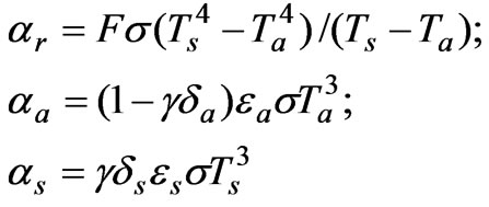 (7)
(7)
Here εa, εs—emissivities of the atmosphere and the ocean; F—transfer factor for the system of the ocean--the atmosphere; δs—the fraction of the ocean emissive power contained in atmospheric windows; δa—the fraction of the atmospheric emissive power contained in atmospheric windows; σ = 5.67·10-8 W/m2K4—the StefanBoltzmann constant; γ—atmospheric transmission for the heat radiation in atmospheric windows.
As it follows from (7), scheme in Figure 1 is considerably nonlinear because the scheme parameters αi depends sharply on the temperatures.
With regard to (6) and (7), system (3) can be expressed as
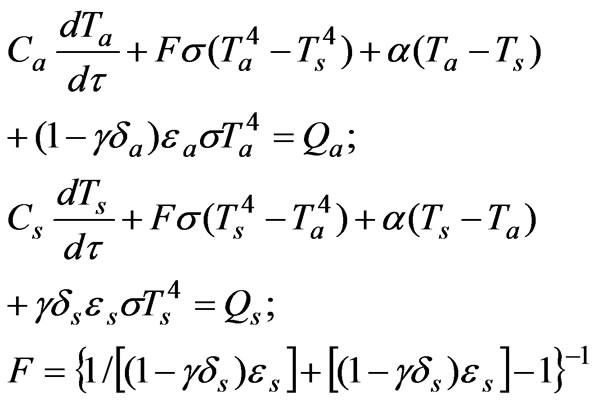 (8)
(8)
To solve the system (8), initial conditions must be adopted, and the set of parameters satisfied to known components of the heat balance Qa, Qs, qs, and Тs must be defined.
It is important to establish the conductivities α correctly. It depends on small variations of Ts and Ta weakly. Arrhenius [4] examined the surface only without analysis of atmospheric temperature situation. He assumed the convective—mass-transfer flux q to be constant. However, as it shows below, condition α = const is more correct. Initial value of α defined from heat transfer equations depends on key parameters included in systems (8) and (5), but it is assumed that α is constant in following calculations of the dependence of Ts and Ta on variations of any parameter.
4. Parameters of Heat Balance for Transient and Steady-State Conditions
Following values were chosen as initial defining components of the heat balance [2] Qs = 168 W/m2; Qa = 67 W/m2; qs = 40 W/m2; qa = 195 W/m2 and Ts = 287K [5]. Surface heat capacity of the atmosphere is obtained from known mass and specific heat capacity of air [3] Cа = 107 J/m2K. For the ocean the heat capacity is obtained throw the specific heat capacity and the density, so Cs = 4.2·106lo, lo is the depth of the ocean mixed layer specified in meters.
Values introduced above are enough to estimate thermal inertia characteristics of the Earth investigated as the whole planet. Impact of parameters variations should be calculated numerically in the non-linear statement of the problem to avoid errors.
We begin with analysis of termoinertia characteristics of the system of the surface—the atmosphere.
Adding up left and right parts of first and second equations from the system (8), we obtain
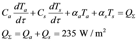 (9)
(9)
For the simplest estimations we assume that the difference between temperatures Ts and Ta is small:
 (10)
(10)
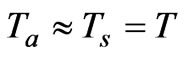
In this case (9) can be introduced in form:
 (11)
(11)
here t—thermal inertia constant for the system of the ocean--the atmosphere; θ—steady-state planetary temperature of the Earth; QΣ—total power of heat sources in the system of the ocean—the atmosphere; αp—planetary conductivity for heat radiation from the Earth to the space.
Equation (11) makes it possible to get the very simple but reliable estimations. It is confirmed by results of our additional non-linear calculations, which makes it seen that the temperature change in time is not strictly exponential, but the duration of the transition condition is estimated exactly with the linear problem definition.
To get estimations, we assume θ ≈ 287K and QΣ = 235 Wm2, and we obtain αp ≈ 0.82 W/m2K. Substituting this value and values of Ca and Cs to formula for the thermal inertia, we find
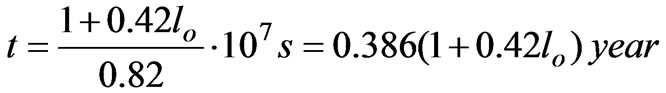 (12)
(12)
Assuming the depth of the ocean mixed layer lo=50 m (accuracy of this value is not so important for demonstrative estimate), the Earth’s thermal inertia constant is obtained to be t = 8.5 years. If any key parameter (atmospheric transmission, solar constant etc.) changes in the spurts manner, the new steady-state condition would form over the time, which approximately equals to three thermal inertia values, in our case τ = 3t = 25.5 years. If key parameters changes slowly then transient process will be much longer.
Next step is to find values of parameters in case of steady-state conditions—when dTi/dτ = 0. We begin with analysis of the connection among transmission γ and emissivities εs and εa.
It is known [3] that main atmospheric window corresponds to the spectral range 8..13 µm. In range 13..17.5 µm the radiation is close to be totally absorbed by CO2 molecules and water vapor (overlap of absorption band-width). In range > 17.5 µm total contribution of transparency lines on order of magnitude in compare with 8..13 µm. We have obtained the energy fraction δ ≈ 0.31 with Ts = 287K. Our calculations have shown that accounting of all atmospheric windows doesn’t change the final result of calculations. From (6) and (7) it is possible to obtain following rate:
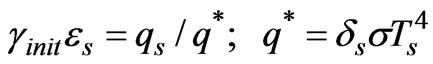 (13)
(13)
here γinit—assumed initial value of transmission, γ is vary relative to it; q*—specific heat flux from the surface with εs =1 to the space throw atmospheric window with absolute transmission γ = 1.
Assuming Ts = 287K and δs = 0.31, we find q* = 120 W/m2. When qs = 40 W/m2 [2] it is following from (13):
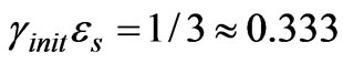 (14)
(14)
From (14) the limitation follows: minimum values γinit and εs equal to 0.333, as γinit ≤ 1 and εs ≤ 1. From (6) and (7) it can be obtained
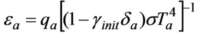 (15)
(15)
There is a problem on this stage. To study the parameters variations impact on the temperatures from the system (8) when dTi/dτ = 0, it is necessary to define initial values of Ta and α which are desired quantity. And we should set initial values of γinit, εs and εa. However, there is indeterminacy as accurate values of these parameters are not known.
To overcome the indeterminacy, we set initial value γ = 0.8 for preliminary calculations. This value looks reliably for the standard atmosphere. Substituting the initial parameter values in the heat balance equations, following values are obtained: Ta = 284.25K; εa = 0.7; α = 45.56 W/m2K. Value εs has been defined from (14) directly. Substituting γinit = 0.8 in (14), we obtain the required value εs = 0.417. This value satisfies the assumed heat flux throw transparency window. Assumed value of εa is arbitrary to a certain extent, but it corresponds to conceptions of planetary heat balance and planetary temperature.
5. Calculations Results
Assuming parameters values, numerical calculations has been performed how the temperatures, the heat fluxes and the heat conductivities depend on atmospheric transmission γ at steady-state conditions.
Plots in Figures 2–4 present these dependencies in all range of transmission change 0 ≤ γ ≤ 1 when conductivity between the ocean and the atmosphere α is constant. Calculations show that in case of constant heat flux q it is the intersection between temperature dependencies. This intersection doesn’t correspond to the assumption q = const. So, we use the assumption α = const in following calculations.
Dependencies of derivatives Ns = dTs/dγ and Na = dTa/dγ on the radiative heat flux from the surface to the space throw atmospheric window were investigated. We found that the decreasing of atmospheric transparency cause the decreasing of Ti when qs < 50 Wm2, because in the range of value 0 < qs < 50 Wm2 the derivatives are positive. For such conditions it is found that decrease of atmospheric transparency (for example, as result of the growing of the greenhouse gases concentration) causes to the increasing of the heat power emitted by the atmosphere to the space,
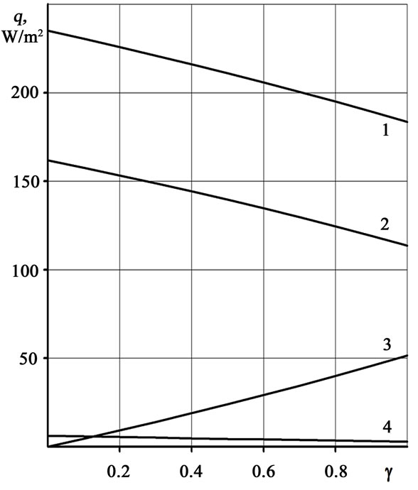
Figure 2. Dependencies of the heat fluxes on atmospheric transmission: 1 – qa; 2 – q; 3 – qs; 4 – qr
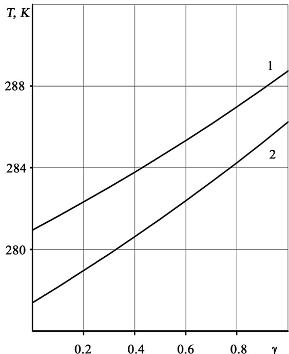
Figure 3. Dependencies of the temperatures on atmospheric transmission: 1 – Ts; 2 – Ta
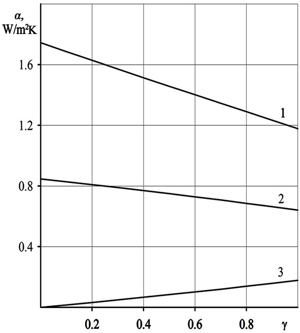
Figure 4. Dependencies of the conductivities on atmospheric transmission: 1 – αr; 2 – αa; 3 – αs
and this heat power increases faster then the heat power absorbed by the atmosphere from the surface radiation. Note, that this result corresponds to conclusion from [6] obtained using the other approach.
Greenhouse effect and global warming in the traditional interpretation take place in the case of the unusually heat fluxes from the surface to the space—when qs > 50 Wm2, and also in case of small initial values of γ. If the inequality εs > εa is satisfied, then decreasing of $\gamma$ would cause warming.
6. Analysis
Dependencies shown in Figures 2–4 are approximated:
For the fluxes:
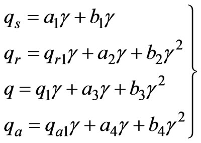 (16)
(16)
For the temperatures:
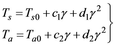 (17)
(17)
For the conductivities:
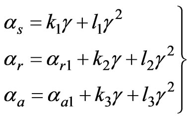 (18)
(18)
Conditions caused by (5) and (16)–(18) should fulfill with any value γ
1) qа – qr – q = Qа = 67 W/m2, from where qа1 – qr1 – q1 + (а4 – а3 – а2)γ + (b4 – b3 – b2)γ2 = 67.\item
2) qs + qа = 235 W/m2 or qа1 + (а1 + а4)γ + (b1 + b4)γ2 = 235.
3) qs + qr + q = 168 W/m2 or q1 + qr1 + (а1 + а2 + а3)γ + (b1 + b2 + b3)γ2 = 168.
4) ΔТ = (Tr – Ta) = (Тs0 – Та0) + (с1 – с2)γ + (d1 – d2)γ2.
From q = αΔТ it follows q1 + a3γ + b3γ2 = α(Тs0 – Та0) + α(с1 – с2)γ + α(d1 – d2)γ2.
q1 = α(Тs0 – Та0); a3 = α(с1 – с2); b3 = α(d1 – d2).
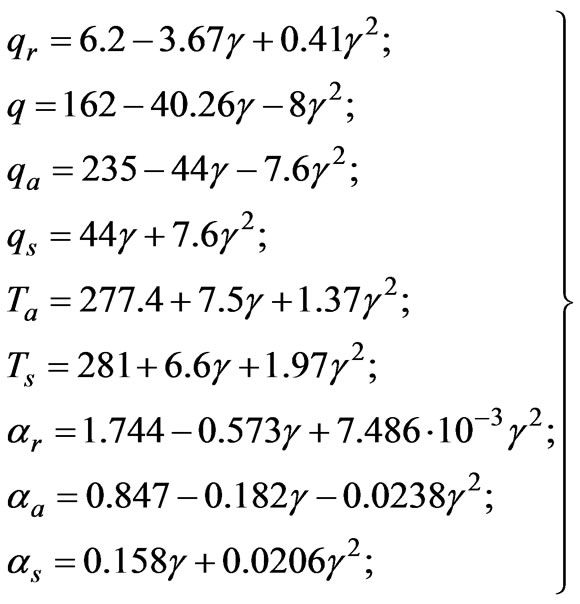
Approximation coefficients are in good agreements with each other. Being round to second sign after dot for the fluxes and the temperatures and to fourth sign after dot for conductivities, its substitution to (16)-(18) makes it possible to get formulas for qualitive calculations with error less then 0.3% (except qs and αs, for its less then 1\%) in form
7. Conclusions
Described research has shown that it is convenient to use the electrical circuit analogy for analysis of the integral heat balance in the system of the surface—the atmosphere—the open space. Reducing of this system to the three-level scheme with lumped parameters (αi) makes the analysis more obvious. This scheme contains some indeterminacy. However, the analytical dependencies connect all coefficients of the radiative heat transfer and specific fluxes with temperatures. So, it is possible to describe the fluxes, temperatures and conductivities as dependencies on any initial parameter. Particularly, its can depend on atmospheric transmission in form (16) –(18).
The parameters γinit and εs are connected by the ratio γinitεs = 1/3, and Ta and εa are connected by the more compound dependence on γinit, so the heat balance contains the indeterminacy in specific values of these parameters. With the more reliable values of listed parameters, there are quantitative dependencies (19).
It is found that if qs ≤ 50 W/m2 and εa > εs then atmospheric transparency decreases and the averaged temperatures decrease. It can be seen from (19) that if γ decreases then qs decreases, but the flux qa from the atmosphere to the open space increases on the same value. Also the atmospheric temperature Ta decreases in spite of increasing of the resultant convective—evaporating flux q. However, q < qa, and the increasing of the flux q can’t compensate the increasing of the flux qa given by the planet to the space. The decreasing of the cover (atmospheric) temperature causes the decreasing of the core (surface) temperature. Anti-greenhouse effect realizes on this way, and the decreasing of atmospheric transmission causes global cooling. It is found as the additional result that the radiative heat transfer qr has small influence on the integral heat balance.
Greenhouse effect in it traditional interpretation realizes when one of the following conditions is satisfied: qs > 50 W/m2; εs > εa; γ < 0.4.
It is found that trends of the climate change caused by the increasing of the carbon dioxide emission depends on the whole set of parameters realized actually nowadays. There is the great interest to determine the values of the parameters as reliably and quickly as possible. Small changes of the basic parameter values established after 12 years [7] don’t influence on our results.
REFERENCES
- J. H. Lienhard IV and J. H. Lienhard V, “A heat transfer textbook,” 3rd Ed., Cambridge, MA, Phlogiston Press, 2008.
- J. T. Keihl and K. E. Trenberth, “Earth’s annual global mean energy budget,” Bulletin of the American Meteorological Society, Vol. 78, No. 2, pp. 197–208, 1997.
- A. P. Babichev, N. A. Babushkina, A. M. Bratkovskii, et al., “Physical values: Handbook energoatomizdat,” I. S. Grigor’eva and E. Z. Melikhova, Ed., Moskow, Russian, 1991.
- S. Arrhenius, “On the influence of carbonic acid in the air upon the temperature of the ground,” Philocophical Magazine and Journal of Science, Vol. 5, No. 41, pp. 237–276, 1896.
- C. N. Hewitt and A. V. Jackson, “Handbook of atmospheric science: Principles and applications,” C. N. Hewitt and A. V. Jackson, Ed., Blackwell Publishing, 2003.
- G. V. Chilingar, L. F. Khilyuk, and O. G. Sorokhtin, “Cooling of atmosphere due to CO2 emission,” Energy Sources, Part A: Recovery, Utilization and Environmental Effects, Vol. 30, pp. 1–9, 2008.
- K. E. Trenberth, J. T. Fasullo, and J. T. Keihl, “Earth’s global energy budget,” Bulletin of the American Meteorological Society, Vol. 90, No. 3, pp. 311–323, 2009.