Journal of Intelligent Learning Systems and Applications
Vol.5 No.1(2013), Article ID:27936,10 pages DOI:10.4236/jilsa.2013.51003
LP-SVR Model Selection Using an Inexact Globalized Quasi-Newton Strategy
![]()
1Department of Computer Science, Baylor University, Waco, TX, USA; 2Department of Electrical and Computer Engineering, Autonomous University of Ciudad Juarez, Ciudad Juárez, Mexico; 3Science Applications International Corporation, El Paso, TX, USA.
Email: Pablo_Rivas_Perea@Baylor.edu, jcota@uacj.mx, jorperez@uacj.mx, dagarcia@uacj.mx, gerardo_rosiles@yahoo.com
Received December 2nd, 2011; revised October 31st, 2012; accepted November 6th, 2012
Keywords: Hyper-Parameter Estimation; Support Vector Regression; Machine Learning; Data Mining
ABSTRACT
In this paper we study the problem of model selection for a linear programming-based support vector machine for regression. We propose generalized method that is based on a quasi-Newton method that uses a globalization strategy and an inexact computation of first order information. We explore the case of two-class, multi-class, and regression problems. Simulation results among standard datasets suggest that the algorithm achieves insignificant variability when measuring residual statistical properties.
1. Introduction
Hyper-parameters estimation is currently one of the general open problems in SV learning [1]. Broadly speaking, one tries to find those hyper-parameters  minimizing the generalization error of an SV-based learning machine. In this regard, Anguita, et al. [2], comments that “the estimation of the generalization error of a learning machine is still the holy grail of the research community.” The significance of this problem is that, if we can find a good generalization error estimate, then we can use a heuristic or mathematical technique to find the hyper-parameters
  via minimization of the generalization error estimate.
Current efforts involve techniques of  -fold cross validation [3], leave-one-out cross validation [2], bootstrapping [4], maximal discrepancy [5], and compression bound [2,6]. However, most algorithms are problem dependent [7]. This statement is confirmed by Anguita, et al. [2]. The authors performed a comprehensive study on the above techniques and they ranked such techniques according to their ability to estimate the true test generalization error. Anguita, et al. [2], concluded that most of the methods they evaluated either underestimate or overestimate the true generalization error. Also, their research suggests that the
  -fold cross validation technique is one of the less risky techniques for estimating the true generalization error.
In this research we use the  -fold cross validation technique to estimate the true test generalization error. Along with this technique, we define error functions as measures of the training generalization error for both classification and regression problems. We propose to minimize the estimated true generalization error by adapting the Newton method with line-search. From the optimization point of view, the solution to the problem is non-trivial. To illustrate this, Figure 1 shows the output root mean squared error of a Linear Programming Support Vector Regression (LP-SVR) as a function of its hyper-parameters
 . Note how the error surface is non-smooth and has many local minima; therefore, it is non-convex. Our aim here is to adapt Newton method to provide an acceptable solution to the problem of finding the hyper-parameters. Although the LP-SVR formulation we discuss here is the one introduced in [8], it will be demonstrated that the method can be implemented for other formulations of support-vector-based problems.
This article is organized as follows: In Section 2, we begin our discussion by defining a generalized method to minimize a set of error functions that will reduce the training generalization error of a generic pattern recognition problem; therefore, in order to demonstrate the potential of this method. Section 3 discusses the usage of an LP-SVR formulation. The latter particularization is addressed in Section 4 where specific error functions are chosen to solve the problem. Section 5 discusses implementation details and other considerations in this research for this particular problem. The results are discussed in Section 6, and conclusions are drawn in Section 7.
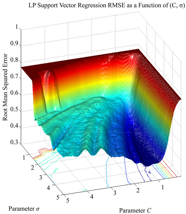
Figure 1. Response of the root mean squared error as a function of . Note, how the error surface is nonsmooth and has many local minima.
2. The Minimization of Error Functions
Let us consider , such that
  and is a real function representing some estimate of error; where
  is a vector of parameters, and
 ![]() defines a training set given by N samples of the M-dimensional data vector
defines a training set given by N samples of the M-dimensional data vector , and a desired output class value
 . Then, let
  be denoted as
 (1)
(1)
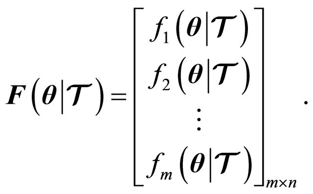
That is,  represents
 ![]() different measures of error, provided model parameters
different measures of error, provided model parameters , and training data
 . Here, we aim to make
![]() .
.
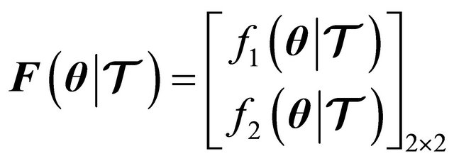
In this paper we will address the case when![]() , that is, when the number of model parameters to estimate, is equal to the number of error metrics used to find such model parameters:
, that is, when the number of model parameters to estimate, is equal to the number of error metrics used to find such model parameters: , and
, and .
.
If , then it has a gradient usually known as Jacobian given by
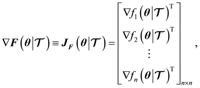 (2)
(2)
where  denotes the gradient of the
 ![]() th function, given by
th function, given by
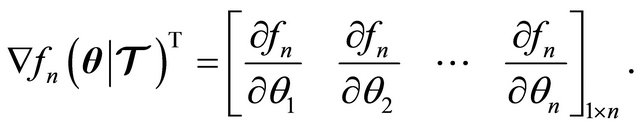 (3)
(3)
Since we want to find the vector of parameters  that given a training set
  produce minimal error functions, such that
 , then we can use Newton’s method assuming, for now, that
  is continuously differentiable on
 .
.
2.1. The Algorithm of Newton
The algorithm of Newton has been used for a number of years; it is well known from basic calculus and is perhaps, one of the most fundamental ideas in any numerical optimization course. This method can be summarized as shown in Algorithm 1.
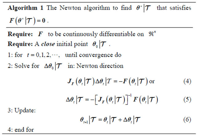
Newton’s method is known because it has q-quadratic rate of convergence, finding a solution  in very few iterations. Such that
 , if and only if such a solution exists.
This method is also known for one of its main disadvantages: it is a local method. Therefore, one need to have in advance a vector of parameters that is close to an acceptable solution. To overcome this difficulty, we can establish a globalization strategy.
2.2. Globalization Strategy
In our globalization strategy we use the following merit function:
 (7)
(7)
where  denotes the
  -norm (a.k.a. euclidean norm). Then we define the following property.
Property 1.  is a descent direction for
  . That is,
  in the system given by
 (8)
(8)
Proof. Let  be the derivative of the merit function (7) denoted as:
 (9)
(9)
Then, substituting (9) into (8) results
 (10)
(10)
which reduces to
 (11)
(11)
Hence, .
.
Given the fact that the merit function (7) is indeed a valid function guaranteeing a descent at every iterate, then, we can establish the globalization strategy by defining the next property.
Property 2. If  is a descent direction of
  , then, there exists an
  such that
 (12)
(12)
The proof for this property is already given by Dennis et al. in 1996 [9] (see Theorems 6.3.2. and 6.3.3. pp. 120-123). Thus, substituting (7) into (12), we obtain
 (13)
(13)
which reduces to
 (14)
(14)
where  is a parameter controlling the speed of the line search. Typically
  [9].
[9].
Using the line-search globalization strategy, we can modify Newton’s method to include a sufficient decrease condition (a.k.a. Armijo’s condition). The Globalized Newton method is as shown in Algorithm 2.

Note that the fact that the algorithm makes progress to an acceptable solution  is due to the new update step (15) that considers the new sufficient decrease condition. In the following sections it is shown how to find parameters from the LP-SVR model.
3. LP-SVR Model Parameters
In this paper we aim to find the parameter of a linear programming support vector regression (LP-SVR) approach, that uses an infeasible primal-dual interior point method to solve the optimization problem [10].
In order to describe the LP-SVR formulation we need to start with the  -SVR. The formulation of an
  - SVR (i.e. norm-1-SVR) problem is as follows:
 (16)
(16)
where ![]() is the Lagrange multiplier associated with the support vectors (SVs); the summation in the cost function accounts for the
is the Lagrange multiplier associated with the support vectors (SVs); the summation in the cost function accounts for the ![]() -insensitive training error, which forms a tube where the solution is allowed to be defined without penalization;
-insensitive training error, which forms a tube where the solution is allowed to be defined without penalization;  is a constant describing the trade off between the training error and the penalizing term
 ; the variable
 ![]() is a nonnegative slack variable that describes the
is a nonnegative slack variable that describes the ![]() -insensitive loss function;
-insensitive loss function; ![]() is the desired output in response to the input vector
is the desired output in response to the input vector![]() ; the variable
; the variable  is a bias;
  is any valid kernel function (see [11,12]). The parameter vector
 ![]() and the bias b are the unknowns, and can take on any real value.
and the bias b are the unknowns, and can take on any real value.
Then, since the requirement of an LP-SVR is to have the unknowns greater than or equal to zero, we typically decompose such variables in their positive and negative parts. Therefore, we denote α = α+ −α−, and b = b+ −b−. Then, in order to pose the problem as a linear program in its canonical form and in order to use an interior point method solver, problem (16) must have no inequalities; thus, we need to add a slack variable u, which alltogether results on the following problem
 (17)
(17)
which is the formulation we used in the analysis we presented in this paper, along with an interior point solver and a radial-basis function (RBF) kernel with parameter![]() .
.
Note that (17) allows us to define the following equalities:
 (18)
(18)
 (19)
(19)
 (20)
(20)
![]() (21)
(21)
which is an acceptable linear program of the form:
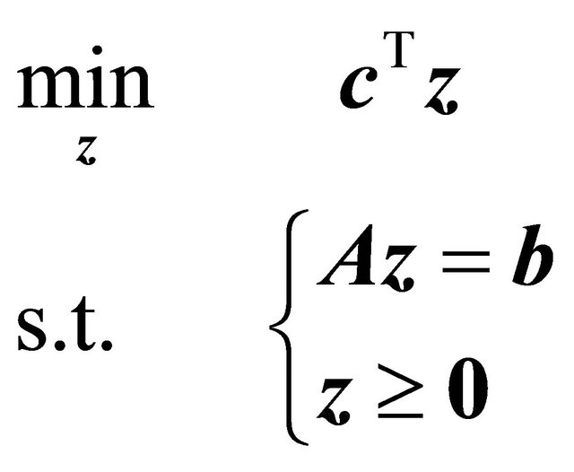 (22)
(22)
Note that this problem has  variables and
  constraints.
This is a definition more appropriate than the one described by Lu et al. in late 2009 [13] for interior point methods; and also it is an extension of the LP-SVM work presented by Torii et al. in early 2009 [14] and by Zhang in early 2010 [15].
Since the LP-SVR definition suffers from an increase in dimensionality, it is suggested that in large scale applications use the approach presented in [8].
4. Error Functions as Model Parameters Selection Criteria
Typically in computational intelligence methods and pattern recognition we want to minimize the true test error. And the true test error has to be measured in some way. The measurement of the test error is in fact modeldependent. In the following paragraphs we will chose error metrics particular to classification and regression problems for the LP-SVR model in (17).
4.1. Error Functions for Two and Multi-Class Problems
In this paper we want to particularize and estimate the model vector of parameters . The error functions we want to use for multi-class problems are two: a modified estimate of sacled error rate (ESER), and the balanced error rate (BER). The ESER metric is given by
 (23)
(23)
where ![]() is a scaling factor used only to match the ESER to a desired range of of values;
is a scaling factor used only to match the ESER to a desired range of of values; ![]() denotes the outcome of the LP-SVR classifier when an input vector
denotes the outcome of the LP-SVR classifier when an input vector ![]() is fed at the LP-SVR’s input; and the function
is fed at the LP-SVR’s input; and the function  is denoted by the following equation:
 (24)
(24)
that approximates the unit step function. The step function is widely used and for this case, the quality of its approximation depends directly of the parameter  as shown in Figure 2.
In all of our experiments  is fixed to
 . If
. If then the f1 has values only within the interval
 .
.
The ESER could become biased towards false positive counts, especially if we have a large number of unbalanced class examples. Therefore, we use the BER which is defined as follows:
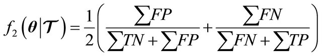 (25)
(25)
where  stands for “True Positive,”
  “False Positive,”
  “True Negative,” and
  “False Negative.” (The reader may find Tables 1 and 2 useful in understanding or visualizing the concepts above using multi-class confusion matrices.)
Whenever there there are equal number of positive and negative examples, which is the case when TN + FP = FN + TP (see [7]), then the BER becomes equivalent to the traditional misclassification rate.
In the other hand, for a two class approach, it is more
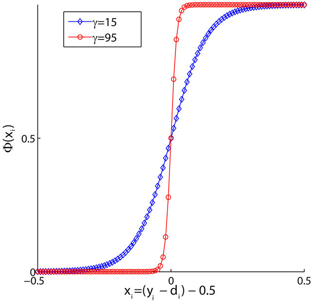
Figure 2. An approximation to the unit step function  was used for convenience in easing computations. A value of of
  provides a better approximation than a value of
 . Larger values for
  produce better approximations to the step function.
Table 1. Illustration of TP, FP, TN, and FN for class 0, using a multi-class confusion matrix.

Table 2. Illustration of TP, FP, TN, and FN for class 2, using a multi-class confusion matrix.

convenient to use the area under the receiver operating characteristic (ROC) curve, as well as the BER metric. It is well known that maximizing the area under the ROC curve (AUC) leads to better classifiers, and therefore, it is desirable to find ways to maximize the AUC during the training step in supervised classifiers. The AUC is estimated by means of adding successive areas of trapezoids. For a complete treatment of the ROC concept and AUC algorithm, please consult [16]. Let us define the function  for the two class approach as follows:
 (26)
(26)
The area under the ROC curve,  , is computed using Algorithms 1, 2, and 3 from [16]. Let us recall that essentially we want
 , which evidently in (26) means a maximization of the AUC. The function
  for the two-class approach is the same BER as in (25).
For regression problems, the error metrics have to be different. The next paragraphs explain functions that can be used.
4.2. Error Functions for Regression Problems
In regression we want to use a different measure of error. The error functions we want to use for classification are two: sum of square error (SSE), and balanced error rate (BER). The SSE metric is given by
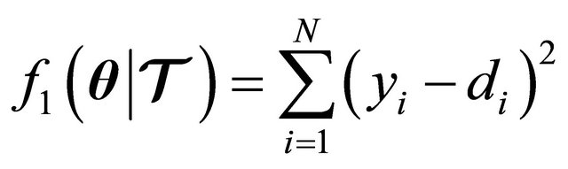 (27)
(27)
where ![]() is the actual output of the classifier LP-SVR when the input vector
is the actual output of the classifier LP-SVR when the input vector ![]() is presented at its input.
is presented at its input.
The second metric is based on the statistical properties of the residual error given by the difference . From estimation theory it is known that if we have the residual error expected value equal to zero, and a unit variance, we have achieved the least-squares solution to the regression problem, either linear or non-linear. Furthermore, it is understood that as the variance of the residual error approaches zero, the regression problem is better solved. Let us denote the expected value of the residual error as
 (28)
(28)
and the variance of the residual error as follows
 (29)
(29)
from where it is desired that . Hence, the second error metric is defined as:
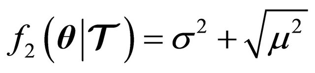 (30)
(30)
where the term  has the meaning of the absolute value of the mean, since
 ![]() is easier to handle in optimization problems.
is easier to handle in optimization problems.
5. Particularization and Discussion
In this section we follow the development presented in Section 2, and cope it with the metrics on Section 4, to find the model parameters of the formulation in Section 3.
5.1. Globalized Quasi-Newton Implementation
Particularizing (1) for the cases presented in Sections 3 and 4, the formulation of  simply becomes
 (31)
(31)
where clearly  and
and . The typical challenge is to compute the Jacobian matrix
 , since not all the error functions are differentiable, i.e. (25) or (26). Then, the classical approaches are to estimate
  via finite difference approximation, or secant approximation. For convenience, we used the finite difference approximation. In this case,
  corresponds to a finite difference derivate approximation which solves (2) using (3) where
 (32)
(32)
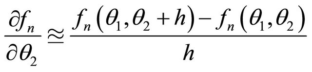 (33)
(33)
allowing  to be sufficiently small, as appropriate.
5.2. Finding a Good Initial Point
Although the globalization strategy presented in Section 3 prevents Newton method from going far away from a solution, and guarantees a decrease of the error at each iteration, it does not guarantees a global minima since it is not a convex problem. As a consequence, we needed to implement a common approach to find the initial vector of parameters, by varying  and
and ![]() and observing for the pair of parameter producing the minimum error. In this paper, this is achieved by varying
and observing for the pair of parameter producing the minimum error. In this paper, this is achieved by varying  in the following interval
  and
and  . In spite that this approach is very powerful to find a good starting point, it requires a loop of
  iterations, which is sometimes very costly depending on the application.
5.3. S-Fold Cross Validation
Estimating the true test error given a training set  is not trivial. Two popular approaches to this problem exist:
 ![]() -fold, and leave-one-out cross validation.
-fold, and leave-one-out cross validation.
In our implementation and experiments, we have used former approach, which led us to define the following rule to find a “good” number of partitions in![]() , that is:
, that is:
 (34)
(34)
where  represents the maximum number of constraints in (22) that are computationally tractable; the function
  represents a round up operation; and
  is the number of partitions in
![]() . In the case of a largescale implementation
. In the case of a largescale implementation  is directly set to the maximum working set size parameter.
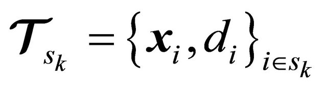
The partitions in the set ![]() is denoted as
is denoted as
 (35)
(35)
where , and
, and  denotes the
  th partition and contains the indexes of those training data points in
![]() . Therefore we say that
. Therefore we say that 
and .
.
It is understood that the main idea behind this method is to partition the training set  in
in  groups of data (ideally of equal size), then train the classifier with
  and use the remaining data as validation set. The process is repeated for all the partitions
  and the error is averaged as follows
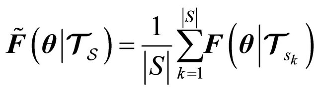 (36)
(36)
where 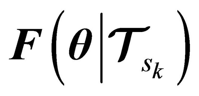 is the error obtained for the
  th partion;
 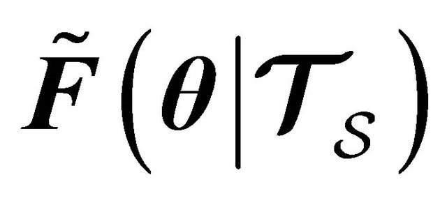 is an estimate of the true test error;
 and
and .
.
5.4. Refined Complete Algorithm
The complete algorithm considering all the refinements and particularizations for the particular case study of the LP-SVR (shown as Algorithm 3) requires as input the indexes S corresponding to the cross validation indexes, and also the training set  from which the LP-SVR parameters producing the minimum error
  will be estimated as
 .
.
Then, the algorithm proceeds using the approximation to the true Jacobian (31)-(33) shown in Section 5.1. However, note that every single function evaluation of (31) requires cross validation, as explained in Section 5.3. As a consequence, the Jacobian implies internal cross validation. The remaining steps are the linear system solution, Armijo’s condition, and update.

The linear system in Step 5.4 requires special attention specially in a large-scale setting. If this is the case, one possible approach is to use any well known direct approach such as LU-factorization [17]; or an indirect approach such as the classic conjugate gradient algorithm by Hestennes 1956 [17,18]. The other special consideration with the linear system is when the Jacobian matrix is non-singular. There is an easy way to test if the Jacobian is non-singular, look for the minimum eigenvalue and if it is less than or equal to zero, then the Jacobian is nonsingular. This idea, leads to a trick that consist on shifting the eigenvalues of the Jacobian so that it becomes singular for computational purposes. With this in mind, we can modify Step 5.4 of the algorithm as follows:
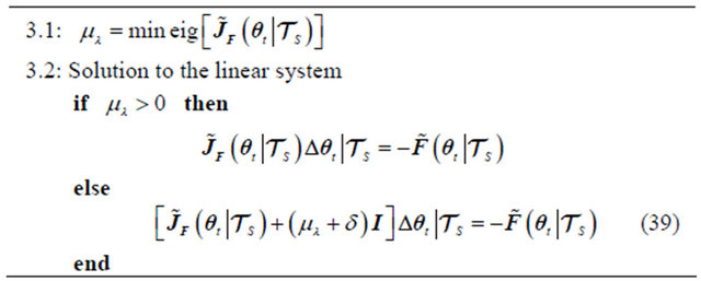
where  is the minimum eigenvalue of the Jacobian,
  is a constant sufficiently small that cannot be interpreted as zero, and
  is the identity matrix of identical size to the Jacobian. In (39) we typically chose
 .
.
5.5. Stopping Criteria
The stopping criteria used in this algorithm includes three conditions.
First, a condition that monitors if the problem has reached an exact solution to the problem, that is,
 (40)
(40)
where . Ideally,
  , and
, and .
.
Second, the  norm of the objective function is monitored, which measures the distance to zero (or to a certain threshold) from an approximate solution at iteration t. That is,
![]() (41)
(41)
where  is some threshold, ideally
 .
.
Third, we set a condition that measures the change between solutions at each iterate, as follows
 (42)
(42)
where  is typically set to a very small value.
Condition (42) states an early stopping criteria if the algorithm has no variability in terms of the updates at each iteration. However, it may happen that the algorithm is indeed changing the solution  at each iterate, but indeed this represent no significant progress towards a solution. In such case, another classical early stopping criteria is used: maximum iterations. The criteria is simply
 (43)
(43)
where  is the maximum number of iterations permitted.
6. Simulation Results
To show the effectiveness and efficiency of the proposed model selection method, we performed simulations over different datasets. The summary of the properties of these datasets are shown in Table 3. Note that the simulations include classification in two and multiple classes, as well as regression problems. The results will be explained in the following paragraphs.
First, let us consider the results shown in Table 4. The second column shows the total number of iterations; in average we observe that the iterations are around eight, which is one of the most important properties of the method. Column three and four of Table 4 show the hyper-parameters found; while in the fifth column we see the  -norm of the algorithm at the last iteration. Note how variable is this value depending on the dataset. Finally, in the sixth column is shown the criteria that made the algorithm stop; it is clear that the most common is the criteria
  described in (42). This latter statement means that the algorithm stopped because no progress was being made towards the solution.
A second part of our the simmulation involves using a testing sed. For this purpose, let us define
 as the testing set, where
  is the number of samples available for testing. The testing set
  has never been showed to the LP-SVR model before.
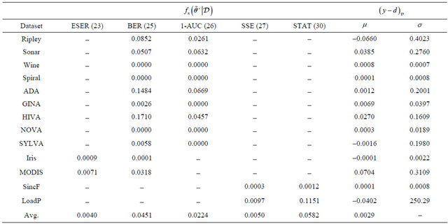
The simulation results in Table 5 show  which represents the result of the
 ![]() -th function (or error criteria), evaluated at the approximated solution
-th function (or error criteria), evaluated at the approximated solution  using only the testing set
 . These results are shown in columns two trough six. In column number two is shown the modified estimate of scaled error rate (23), which was used with parameters
  and
and . These parameter
 ![]() was chosen by convenience in order to have an error within the interval [0,1]. The third column displays results for when the balanced error rate (25) was utilized. The area under the ROC curve (26) shown in the fourth column also produces a result within the same interval as the BER. In contrast, regression error functions shown in the fifth and sixth column have a wide interval, but is always positive. That is, sum of squared error (27) and the statistical properties (30) fall into the interval
was chosen by convenience in order to have an error within the interval [0,1]. The third column displays results for when the balanced error rate (25) was utilized. The area under the ROC curve (26) shown in the fourth column also produces a result within the same interval as the BER. In contrast, regression error functions shown in the fifth and sixth column have a wide interval, but is always positive. That is, sum of squared error (27) and the statistical properties (30) fall into the interval . Note that classification error functions in average are zero for practical purposes, which is desirable.
Moreover, in Table 5 columns six trough seven we show statistical properties of the residuals given by . This residual is acquired by showing the testing set
  to the LP-SVR model with hyper-parameters
  and measuring the output
![]() . Ideally, we want the average of the residuals to be zero, as well as their standard deviation. This desired property is achieved during our simulations.
. Ideally, we want the average of the residuals to be zero, as well as their standard deviation. This desired property is achieved during our simulations.
Although statistical properties of residuals based on the testing set demonstrate that the approach has an acceptable behavior, the reader must be aware that this approach has some characteristic properties that may lead
Table 3. Summary of the dimensions and properties of the datasets.

Table 4. Summary of behavior.

to unexpected results. First, the algorithm works with an approximation to first order information, that in the worst case may also be singular. Second, the algorithm is not convergent to a global minimum; however a “good” initial point is obtained as explained in Section 5.2. Third, the globalization strategy may become computationally expensive if the first order information leads far away from the solution. A good way to reduce the computational expense in finding a  that produces a sufficient decrease at each iterate can be found in text books [9,17]; in these, the most common state-of-the-art approach is is to have
  decrease in the following pattern
 . This approach has demonstrated to be efficient and is widely used in the community. However, further research must be conducted in the three aspects mentioned above.
Furthermore, different or more error functions may also be studied we well as the case when more LP-SVR parameters are being estimated, such as![]() . Moreover, the concepts discussed in this paper can also be applied
. Moreover, the concepts discussed in this paper can also be applied
Table 5. Summary of Experiments. Note that the symbol “![]() ” indicates that the error function does not apply to that particular dataset depending if it is multi-class, regression, or two-class.
” indicates that the error function does not apply to that particular dataset depending if it is multi-class, regression, or two-class.
to other support vector (SV)-based learning machines with little or no modification.
7. Conclusions
An algorithm for LP-SVR model selection has been discussed in this paper. We propose a quasi-Newton method for function minimization, that uses a globalization strategy and an inexact computation of first order information. This Jacobian is computed via finite differences techniques. We have explored the case of two and multiclass problems including regression.
Simulation results suggest that the algorithm achieves insignificant variability when measuring residual statistical properties. These simulations included mostly standard benchmark datasets from real-life applications, and fewer synthetic datasets.
This paper discussed discussed a particularization of a generalized method that was introduced at the beginning of this paper; this method can be used to train other types of SV-based formulations. This research significantly advances the natural problem of model-selection in most of today’s SV-based classifiers that have the hyper-parameters out the problem formulation.
8. Acknowledgements
The author P. R. P. performed part of this work while at NASA Goddard Space Flight Center as part of the Graduate Student Summer Program (GSSP 2009) under the supervision of Dr. James C. Tilton. This work was supported in part by the National Council for Science and Technology (CONACyT), Mexico, under Grant 193324/ 303732 and mentored by Dr. Greg Hamerly who is with the department of Computer Science at Baylor University. Finally, the authors acknowledge the support of the Large-Scale Multispectral Multidimensional Analysis (LSMMA) Laboratory (www.lsmmalab.com).
REFERENCES
- A. J. Smola and B. Scholkopf, “A Tutorial on Support Vector Regression,” Statistics and Computing, Vol. 14, No. 3, 2004, pp. 199-222. doi:10.1023/B:STCO.0000035301.49549.88
- D. Anguita, A. Boni, S. Ridella, F. Rivieccio and D. Sterpi, “Theoretical and Practical Model Selection Methods for Support Vector Classifiers,” Support Vector Machines: Theory and Applications, Vol. 177, 2005, pp. 159-179. doi:10.1007/10984697_7
- K. Duan, S. Keerthi and A. Poo, “Evaluation of Simple Performance Measures for Tuning SVM Hyperparameters,” Neurocomputing, Vol. 51, 2003, pp. 41-59. doi:10.1016/S0925-2312(02)00601-X
- Z. Hui-ren and P. Zheng, “Method for Selecting Parameters of Least Squares Support Vector Machines Based on GA and Bootstrap,” Journal of System Simulation, Vol. 12, 2008.
- D. Anguita, S. Ridella, F. Rivieccio and R. Zunino, “Hyperparameter Design Criteria for Support Vector Classifiers,” Neurocomputing, Vol. 55, No. 1-2, 2003, pp. 109- 134. doi:10.1016/S0925-2312(03)00430-2
- L. Wang and S. O. Service, “Support Vector Machines: Theory and Applications,” Studies in Fuzziness and Soft Computing, Springer-Verlag, Berlin, 2005.
- G. Cawley, “Leave-One-Out Cross-Validation Based Model Selection Criteria for Weighted Ls-Svms,” IEEE International Conference on Neural Networks, 16-21 July 2006. doi:10.1109/IJCNN.2006.246634
- P. R. Perea, “Algorithms for Training Large-Scale Linear Programming Support Vector Regression and Classification,” Ph.D. Thesis, The University of Texas, El Paso, 2011.
- J. Dennis and R. Schnabel, “Numerical Methods for Unconstrained Optimization and Nonlinear Equations,” Society for Industrial Mathematics, 1996. doi:10.1137/1.9781611971200
- M. Argaez and L. Velazquez, “A New Infeasible InteriorPoint Algorithm for Linear Programming,” Proceedings of the 2003 Conference on Diversity in Computing, ACM, New York, 2003, pp. 12-14. http://doi.acm.org/10.1145/948542.948545
- J. Mercer, “Functions of Positive and Negative Type, and Their Connection with the Theory of Integral Equations,” Philosophical Transactions of the Royal Society of London. Series A, Containing Papers of a Mathematical or Physical Character, Vol. 209, No. 441-458, 1909, pp. 415-446. doi:10.1098/rsta.1909.0016
- R. Courant and D. Hilbert, “Methods of Mathematical Physics,” Interscience, New York, 1966.
- Z. Lu, J. Sun and K. R. Butts, “Linear Programming Support Vector Regression with Wavelet Kernel: A New Approach to Nonlinear Dynamical Systems Identification,” Mathematics and Computers in Simulation, Vol. 79, No. 7, 2009, pp. 2051-2063. doi:10.1016/j.matcom.2008.10.011
- Y. Torii and S. Abe, “Decomposition Techniques for Training Linear Programming Support Vector Machines,” Neurocomputing, Vol. 72, No. 4-6, 2009, pp. 973-984. doi:10.1016/j.neucom.2008.04.008
- L. Zhang and W. Zhou, “On the Sparseness of 1-Norm Support Vector Machines,” Neural Networks, Vol. 23, No. 3, 2010, pp. 373-385. http://www.sciencedirect.com/science/article/B6T08-4XVBP5J-1/2/b032646ea72f40e7025a40b499134a21
- T. Fawcett, “Roc Graphs: Notes and Practical Considerations for Researchers,” Machine Learning, Vol. 31, 2004, pp. 1-38.
- J. Nocedal and S. Wright, “Numerical Optimization,” Springer Verlag, New York, 1999. doi:10.1007/b98874
- M. Hestenes, “Pseudoinversus and Conjugate Gradients,” Communications of the ACM, Vol. 18, No. 1, 1975, pp. 40-43. doi:10.1145/360569.360658