Wireless Sensor Network
Vol.5 No.4(2013), Article ID:30914,6 pages DOI:10.4236/wsn.2013.54011
Improved Enhanced Chain Based Energy Efficient Wireless Sensor Network
1Computer Science and Engineering, ITM University, Gurgaon, India
2Electronics and Communication Engineering, Guru Nanak Dev University, Amritsar, India
Email: shilpa.kaushal@gmail.com
Copyright © 2013 Shilpa Mahajan et al. This is an open access article distributed under the Creative Commons Attribution License, which permits unrestricted use, distribution, and reproduction in any medium, provided the original work is properly cited.
Received February 12, 2013; revised March 13, 2013; accepted March 28, 2013
Keywords: Energy Conservation; Network Lifetime; Chain Based; ECBSN; Distance
ABSTRACT
In this paper, we have proposed an energy efficient chain based protocol which is an improvement over ECBSN (Energy Efficient Chain Based Sensor Network). ECBSN protocol has certain deficiencies like the non optimal selection of leader nodes in rounds, aggregation and transmission of data by head nodes that leads to unbalanced energy consumption. Aiming at these problems, an improved chain based protocol is proposed. IECBSN adopts a new method of selection of leader nodes based on selection value (SV) parameter .To lower energy consumption further, one more level of hierarchy has been added with a head leader node, which will aggregate data from the leader nodes and pass it to the base station. IECBSN shows an improvement of 20% - 35% as compare to PEGASIS (Power Efficient Gathering in Sensor Information System) and 5% t to 7% from ECBSN on energy consumption and improves network lifetime.
1. Introduction
Wireless sensor network (WSN) is a large network of sensor nodes and these nodes are directly interacting with the environment by sensing physical parameters such as temperature, humidity etc. All the sensor nodes send and receive data to/from a fixed wired station called base station (BS). The base station usually serves as a gateway to some other network. It has wide range of applications ranging from military, environmental, home security etc. The main challenge is related to the limited, usually unrenewable energy supply of the sensor nodes. Hence, the available energy at the nodes should be considered as a major constraint while designing the routing protocols.
In the network model, hierarchical routing protocol is very adapted. Nodes reduce redundancy by aggregating data locally, and leader nodes collect the data gathered from multiple nodes and then send it to the Base Station. In our proposal we have proposed a new routing protocol and it uses the similar radio model as described in [1].
IECBSN, a hierarchical chain based protocol in which sensor nodes are grouped into parallel chains using the minimum distance criteria. A selection value parameter has been defined for selecting leader nodes. One more level of hierarchy has been added for head leader node.
The remainder of the paper is organized as follow: In Section 2 presents the overview of the related works. The network and radio model of our proposal is discussed in Section 3. The details of IECBSN protocol, an analysis and simulation is followed by comparative analysis is discussed in Section 4. Finally Section 5 concludes the paper.
2. Related Work
Both LEACH (Low Energy Adaptive Clustering Hierarchy) protocol presented in [2] and PEGASIS protocol in [3] are popular cluster-based routing protocols which provide elegant solution to minimize energy dissipation and to prolong the network lifetime. In LEACH, cluster heads randomly rotate in order to balance the network energy dissipation. However, the drawback of LEACH is that the dynamic cluster formation causes a massive overhead that increases the network energy dissipation. PEGASIS protocol in [4] improves LEACH on energy efficiency and lengthen network lifetime. It is different from the multi-cluster topology of LEACH that PEGASIS organizes sensor nodes into a chain so that the sensor node on a chain can communicate with one neighbor and only one node can be chosen as cluster head to sent data to the end user. This protocol has shown a better performance than LEACH. However, there are still some limitations in PEGASIS. Firstly, the chain topology introduces excessive delay that causes collection of data out of date. Secondly, the greedy algorithm can keep the minimum distance of each hop while it can not achieve the optimal routing in the whole network. Thirdly, the single cluster-head may become a bottleneck.
Considerable amount of research has been done on chain based protocols and numbers of schemes have been devised. Like [5] an energy efficient level based approach has been proposed in this, a network area has been partitioned into annular rings by using various power levels at the base station and each ring having various sensor nodes. In [6] the author proposes PEGASIS based protocol, in which each node has been assigned a weight so as to represent its appropriate level of being a leader. It considers distance and energy as the key parameter while selecting the leader.
CRBCC [7] gives a good compromise between energy consumption and delay. Chains are formed based on simulated annealing (SA) algorithm. Clusters are formed based on y co-ordinate and chain leaders are formed on x co-ordinates.
A new routing and gathering approach [8] in which clusters are formed and cluster head selected using LEACH approach and then in the clusters, chains are formed using shortest path first. Clusters and chain construction occurs only once and the cluster head rotates locally inside the cluster without re clustering.
In [9], an author proposes a distributed chain based approach routing scheme, in which the entire network area is divided into equal size sub areas. The nodes in these subareas are connected forming chains using minimum spanning tree approach. The sub networks are connected using bridge nodes.
ECBSN [10,11] overcomes several problems of PEGASIS. It overcomes the problem of excessive delay, instead of one long chain in the network number of short chains are formed. In ECBSN, every first node in a chain becomes a leader node. Thus, it ignores the suitable proportion of nodes energy and distance between node and base station which optimize the leader selection according to the various application environments.
Based on the above analysis, this paper presents an improved technique over ECBSN with balanced energy consumption by selecting a leader node considering both energy and distance factor. The results show IECBSN outperforms ECBSN on reduced energy consumption.
3. Network Model
Comparison Chart (Table 1)
The following network model assumptions are considered while constructing IECBSN:
• The BS is located far from the sensor network and fixed.
• All nodes are homogeneous and energy constrained.
• Data are collected periodically from the network and delay critical.
• Radio channel is symmetric so that the energy required to transmit a message from node i to node j is the same as energy required to transmit a message from node j to node i for a given signal to noise ratio.
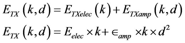
For the sake of uniformity it uses the same radio model as used in LEACH and PEGASIS. The energy consumed in transmitter amplifier for transmission is 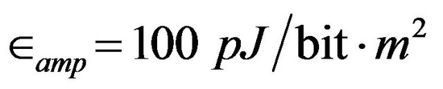 for a decent signal to noise ratio (SNR). In addition energies required in running transmitter and receiver electronics are equal and given by:
 .
.
Thus for free space model, the total transmission cost for a k-bit message to transmit to a distance d is given by the Equation (1).
 (1)
(1)
The energy consumption in the receiver is given by Equation (2).
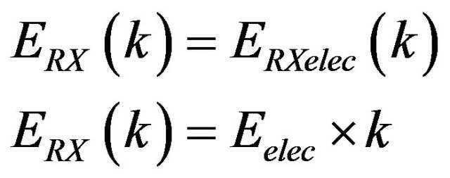 (2)
(2)
Moreover, the energy cost for data aggregation is considered as 5 nJ/bit/message.
Table 1. Comparison of protocols (discussed above).

4. Description of IECBSN
IECBSN is an improved chain based routing algorithm over ECBSN. It is operating by rounds which contain four main phases; Network construction phase, Chain construction phase, leader selection phase and data transmission phase.
4.1. Network Construction Phase
In network construction phase, a 100m × 100m network area in which 100 nodes are densely deployed has been considered. Each node calculates a known distance from the origin. A maximum distance node will be treated as a base station. A chain formation starts from a base station node. In chain formation phase different level chains are formed and in data transmission phase information is transmitted along with the designated paths. We assume that a position from a base station to every node is known based on the received radio signal strength. A node selection procedure (discussed below) is executed to find all the active nodes that take part in the chain formation process (Figure 1).
• 4.2. Node Selection Procedure
• Initialize all the network parameters .Determine the number of nodes, initial energy, BS location.
• Then chain construction starts from the base station (Node at the maximum distance from the origin).
• A source node S broadcast a route request hello message to obtain the distance of each node from S.
○ For neighbors n1, n2, n3···.
○ Compare dist (n1), dist(n2), dist(n3)··· from a source node (S).
○ Active Reply is generated containing route length.
○ Where, dist(n), distance of a neighbor n from the Source node.
• At the source node S
○ All received REPLY messages are scanned.
○ The neighbor with shortest active route is selected for forwarding the data.
• The selected neighbor will act source for other nodes which have not joined the chain yet.
• Continue until all nodes have been traversed.
4.3. Construction Phase
For a N Node network, if each chain contain M nodes. The number of chains formed are (P = N/M). A node in a chain selects the nearest node that has not been yet selected based on the criteria discussed above (node selection procedure). The chain formation continues until all the active nodes are grouped into chains (refer: chain formation algorithm).
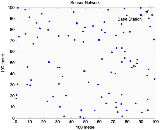
Figure 1. 100 × 100 meter network constructed with base station in Matlab 7.0.
4.4. Chain Formation Phase
1) Initialize node number = N.
2) Initialize chain length = M.
3) Number of chains (P = N/M).
4) Start from the base station, using node selection procedure an active node will be selected.
5) Initialize c = 0 (chain counter).
6) c = c + 1.
7) The selected node will act as a source node for other nodes (Follow Node selection procedure).
8) Repeat steps 6 and 7 while (c ≤ M).
9) Repeat steps 5-7 till all the chains are formed ≤ P.
4.5. Leader Selection Phase
After fixing the chains the next target is to find out the leader node in a chain. This protocol will choose leader based on the Selection Value parameter (SV).
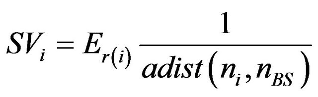
Where Er(i) = residual energy of a node in a chain. Here, residual energy corresponds to Energy of a node in a particular Round (r)-Energy consumed by a node (i) in transmission of data to the base station.
adist(ni, nBS) = distance of a node i to the base station.
• In a chain, Calculate SV for each node and compare If SVi > SVj where SVi and SVj are the selection values of nodes. SVi, node will get selected as leader
• Repeat this process for all chains (≤p) in a network
• The leader nodes will aggregate data from the neighboring node in a chain.
4.6. Data Transmission Phase
After the formation of the chain and selection of leaders, the data transmission phase starts. We assume that sensors always have data to send to the base Here in Figure 2, an area of 100 meter x100 meter network has been taken, it can be clearly seen that both in ECBSN and IECBSN, number of chains with node length four have been formed .The selection of leader node differs in both ECBSN and IECBSN. In ECBSN every first node in a chain has been selected as leader node (indicated by + sign) whereas selection of leader node in IECSBN depends upon SV parameter. Also, an extra level of hierarchy has been added in order to decrease the distance between the leader nodes and base station. Among the leader nodes, a leader node which is at the minimum distance to the base station will act as a head leader node. Head leader node will aggregate all the data from the leader nodes and pass it to the base station.
5. Simulation and Results
In simulation, we have considered a random network of nodes placed in an area. Initially all the nodes have same amount of initial energy. A simulation is performed on mat lab 7.0 considering first radio model. To evaluates

Figure 2. ECBSN and IECBSN network in MATLAB.
the performance of the proposed scheme; we have compared proposed protocol with the PEGASIS and ECBSN.
We assume that 100 sensor nodes are randomly deployed over 100 × 100 m square area field. The base station is located at (97, 100).The initial energy of each node is 0.5 J and node is considered dead when its energy is less than or equal to zero as shown in Table 2.
As discussed, It can be clearly seen that in ECBSN every first node in a network has been taken as leader node (indicated by “+”) but in IECBSN, the leader nodes are selected based on SV criteria which considers both the residual energy and distance parameters into consideration. Also, We know that energy is directly proportion to the (distance)2 ,thus by introducing the head leader node a distance factor has been further reduced. All these measure results in reduced energy consumption and thus increases the lifetime of the network.
5.1. Evaluation of IECBSN with PEGASIS and ECBSN by Varying Node Number
Figure 3, shows the total energy consumed in a network by varying the number of nodes in a network. The simulations have been carried out by varying number of nodes as 20, 32, 52, 72, 100, 150··· For this paper, we have taken a chain of node length four. In order to get appropriate results we have considered node numbers in a multiple 4. The simulation has been carried out for 10 rounds. The results shows the proposed algorithm performs better when compared with a base protocol PEGASIS and ECBSN.
5.2. Energy Consumption vs Rounds
Total energy consumed in a network has been found out by running the simulation for different number of rounds In this paper we have defined .Extensive simulation has been carried out to get the best results, by varying rounds for 30, 50, 100, 150, 200, 350, 500. Nodes considered are 100.The result shows the energy consumption of proposed protocol is much lower as compare to PEGASIS and ECBSN.
Table 2. Network specifications.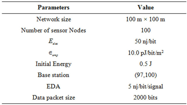
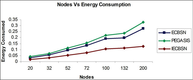
Figure 3. Energy consumption vs nodes.
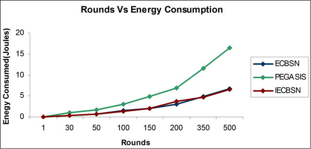
Figure 4. Energy consumption vs rounds.
Here, it can be seen from Figure 4 that IECBSN shows 20% to 35% than PEGASIS .And IECBSN shows 5% to 7% improvement from ECBSN.
5.3. Life Time of WSN
The result between the number of node alive and the number of rounds is shown. The result obtained by measuring the time until the first node dies .We compare both the protocols and found out that in a proposed protocol the nodes death is delayed where as in Pegasis the nodes start to die earlier in rounds as compared to proposed protocol. Also, it can be seen that Nodes dies earlier in ECBSN as compare to IECBSN (Figure 5).
5.4. Number of Dead Nodes
Life time of a network can also be evaluated based upon the number of dead nodes. It has been found that nodes die earlier in PEGASIS and ECBSN when simulation is performed for different number of rounds (Figure 6).
6. Conclusion
In this paper we have proposed IECBSN protocol which is an improved energy efficient PEGASIS based protocol in order to perk up the deficiencies of ECBSN protocol. This protocol adopts a more novel approach for leader selection based on distance and energy criteria. This process even results in balanced energy consumption by considering selection of head leader node for transmission and aggregation of data, which outperforms ECBSN .Considering all these factors, the proposed protocol shows a remarkable improvement over existing

Figure 5. Life time of a network.
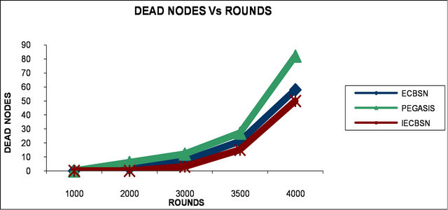
Figure 6. Dead node comparison.
protocols. In future work we can further extend this to multiple layer hierarchical chain based protocol. This can be enhanced further by including issues of MAC layer like active/sleep cycle.
REFERENCES
- S. IAkyildiz and Y. Sankarasubramaniam, “Wireless Sensor Networks: A Survey,” IEEE Computer Networks, Vol. 38, No. 4, 2002, pp. 393-422.
- Heinzelman and B. Krishnan, “An Application-Specific Protocol Architecture for Wireless Micro-Sensor Networks,” IEEE Transactions on Wireless Communicationss, Vol. 1, No. 4, 2002, pp. 660-670.
- S. Lindsey and C. Raghavendra, “PEGASIS: Power-Efficient Gathering in Sensor Information Systems,” IEEE Aerospace Conference Proceedings, Vol. 3, 2002, pp. 1125- 1130. doi:10.1109/AERO.2002.1035242
- Y. Y. Liu, H. Ji and G. X. Yue, “An Energy-Efficient PEGASIS-Based Enhanced Algorithm in Wireless Sensor Networks,” China Communication, 2006, pp. 1-4.
- M. Diwakar and S. Kumar, “An Energy Efficient Level Based Clustering Routing Protocol for WSN,” International Journal of Aeronautical and Space Sciences, Vol. 2, No. 2, 2012, pp. 55-64
- F. Sen and J. Bing, “An Improved Energy Efficient PEGASIS-Based Protocol in Wireless Sensor Network,” 8th International Conference on Fuzzy System and Knowledge Discovery (FSKD), Shanghai, 26-28 July 2011, pp. 2230-2233.
- G. S. Zheng and Z. B. Hu, “Chain Routing Based on Co- Ordinates-Oriented Strategy in WSN,” Proceeding in Computer Networks and Multimedia Technologies, Wuhan, 18-20 January 2009, pp. 1-4.
- J. Duck, et al., “An Efficient Chain-Based Clustering Routing Protocol for WSNs,” International Conference on Advanced Information and Application Workshops, Bradford, 26-29 May 2009, pp. 383-388.
- K. S. Ahn and O. Song, “Balanced Chain Based Routing Protocol (BCBRP) for Energy Efficient Wireless Sensor Network,” IEEE International Symposium on Parallel and Distributed Processing with Application Workshop (ISPAW), Busan, 26-28 May 2011, pp. 227-231.
- S Mahajan and J. Malhotra, “Energy Efficient Path Determination in Wireless Sensor Network Using BFS Approach,” Wireless Sensor Network, Vol. 3, No. 11, 2011, pp. 351-356. doi:10.4236/wsn.2011.311040
- S. Mahajan and J. Malhotra, “Enhanced Chain Technique Based Data Collection Sensor Network,” International Journal of Computer Science, Vol. 8, No. 3, 2011, pp. 83- 87.