Journal of Water Resource and Protection
Vol.6 No.8(2014), Article
ID:47013,16
pages
DOI:10.4236/jwarp.2014.68072
Mapping Mountain Front Recharge Areas in Arid Watersheds Based on a Digital Elevation Model and Land Cover Types
E. E. Bowen1*, Y. Hamada1, B. L. O’Connor2
1Environmental Science Division, Argonne National Laboratory, Argonne, USA
2Department of Civil and Materials Engineering, University of Illinois at Chicago, Chicago, USA
Email: *ebowen@anl.gov
Copyright © 2014 by authors and Scientific Research Publishing Inc.
This work is licensed under the Creative Commons Attribution International License (CC BY).
http://creativecommons.org/licenses/by/4.0/


Received 5 May 2014; revised 1 June 2014; accepted 16 June 2014
ABSTRACT
A recent assessment that quantified potential impacts of solar energy development on water resources in the southwestern United States necessitated the development of a methodology to identify locations of mountain front recharge (MFR) in order to guide land development decisions. A spatially explicit, slope-based algorithm was created to delineate MFR zones in 17 arid, mountainous watersheds using elevation and land cover data. Slopes were calculated from elevation data and grouped into 100 classes using iterative self-organizing classification. Candidate MFR zones were identified based on slope classes that were consistent with MFR. Land cover types that were inconsistent with groundwater recharge were excluded from the candidate areas to determine the final MFR zones. No MFR reference maps exist for comparison with the study’s results, so the reliability of the resulting MFR zone maps was evaluated qualitatively using slope, surficial geology, soil, and land cover datasets. MFR zones ranged from 74 km2 to 1547 km2 and accounted for 40% of the total watershed area studied. Slopes and surficial geologic materials that were present in the MFR zones were consistent with conditions at the mountain front, while soils and land cover that were present would generally promote groundwater recharge. Visual inspection of the MFR zone maps also confirmed the presence of well-recognized alluvial fan features in several study watersheds. While qualitative evaluation suggested that the algorithm reliably delineated MFR zones in most watersheds overall, the algorithm was better suited for application in watersheds that had characteristic Basin and Range topography and relatively flat basin floors than areas without these characteristics. Because the algorithm performed well to reliably delineate the spatial distribution of MFR, it would allow researchers to quantify aspects of the hydrologic processes associated with MFR and help local land resource managers to consider protection of critical groundwater recharge regions in their development decisions.
Keywords:Water Resources, Arid Environment, Groundwater Recharge, Mountain Front, GIS

1. Introduction
Groundwater in the southwestern United States is limited by arid and semiarid climates, rising regional water demand, and potentially increasing climate variability. This resource is replenished through groundwater recharge, a process that is affected by the expansion of land development. Development that creates impermeable surfaces alters rainfall-runoff dynamics and the location and magnitude of infiltration by changing land cover and soil properties that control recharge processes [1] [2] . Today, the rapid growth of energy production facilities is one significant driver of land development in the western United States [3] [4] . The US Department of Energy (DOE), Energy Efficiency and Renewable Energy Program, and the US Department of the Interior, Bureau of Land Management (BLM), released the Solar Programmatic Environmental Impact Statement (Solar PEIS) in 2012 [5] , which evaluated a range of potential development options for production of utility-scale solar energy on federal lands in the southwestern United States. One of the options examined in the PEIS was to focus development of solar facilities in selected areas called solar energy zones (SEZs) that are located in large arid and semiarid basins in order to limit environmental impacts. As a part of the PEIS, an assessment of groundwater resources was conducted for individual SEZs. This assessment necessitated the development of a methodology to identify locations of mountain front recharge (MFR) in order to facilitate land development decisions that would minimize impacts on ground water recharge occurring at the mountain front.
Minimizing impacts on MFR is important because it is a dominant mechanism for groundwater recharge from surface water infiltration in aquifer-stream systems in arid regions. In total, MFR contributes from one-third to nearly all groundwater recharge in arid, mountainous basin fill aquifers depending on local physiographic conditions, and is often the single largest contribution [6] -[9] . Recharge can be increased at the mountain front compared with the upstream mountain face because its unconstrained, depositional setting facilitates higher rates of water infiltration [10] . Infiltration can also be higher at the mountain front compared with the downstream basin floor because snowmelt-driven flow from higher elevations tends to be greater than precipitation received directly by the basin floor [11] . As a result, groundwater recharge can be greater at the mountain front than in higher elevation mountain locations or the valley bottom.
While the importance and mechanisms of MFR are well documented, locations of MFR have not been described in a spatially explicit manner. Studies conducted by Burness et al. [12] and Covino and McGlynn [7] quantified MFR as a component of the water balance, in particular hydrologic systems; however, its specific geographic distribution within the watershed was not identified. In addition, a number of prior geomorphological works examined characteristics of depositional landforms and their formational processes in arid, mountainous watersheds using geographic information system (GIS) tools [13] -[15] . Although these features are closely related to MFR in the landscape, the methods used by these authors were not applied to study MFR directly. Ultimately, none of these studies examined the geographic distribution of MFR itself.
In this study, the geographic distribution of MFR was mapped using a conceptual model of hydrology associated with MFR at a basin level, coupled with terrain analysis techniques. The concept for a spatially explicit definition of MFR has been gradually emerging. A widely recognized topographical definition of MFR [16] identified areas where MFR occurs as being coincident with the piedmont region between the mountain face and basin floor. In addition, recent studies in terrain analysis and geomorphology have demonstrated advanced understanding of landforms, including the piedmont region that is associated with MFR [17] -[23] . However, mapping MFR zones by linking these recent efforts has not yet been attempted. The objective of this study was to develop a systematic, spatially explicit algorithm for generating MFR zone maps in arid and semiarid regions of the southwestern United States based on slope and land cover types by applying the conceptual and methodological approaches in existing research.
2. Study Area
The analysis focused on study watersheds of 17 SEZs across six states—Arizona, California, Colorado, Nevada, New Mexico, and Utah (Table 1)1. Watersheds for this study were defined as the single or multiple 10-digit hydrologic unit code (HUC10) watersheds overlying each SEZ. Watersheds were chosen as the unit of analysis for the purpose of including the basin and piedmont regions in the vicinity of each SEZ included in the analysis. Surface area, elevation, and climatic conditions were identified for the 17 SEZs and study watersheds. The HUC8 watersheds in which SEZs are located were also identified. Surface area of the study watersheds ranged from 555 km2 (for Four mile East in Colorado) to 4205 km2 (for Riverside East in California). Elevations near SEZs ranged from −4 m (Imperial East in California) to 4365 m above mean sea level (Four mile East in Colorado).
Thirteen of the 17 watersheds are located in the Basin and Range US Geological Survey (USGS) Physiographic Province, while the four Colorado watersheds are located in the Southern Rocky Mountains USGS Physiographic Province [24] (Figure 1). The Basin and Range province is an expansive area of north-south-oriented faulted mountains with flat, arid, or semiarid valleys. Basin and Range watersheds in this study have hot desert

Table 1 . Climatic and ecological characteristics of the 17 SEZs and study watersheds.
a8-digit hydrologic unit code; bMeters above mean sea level; cClimate data from western regional climate center [38] .
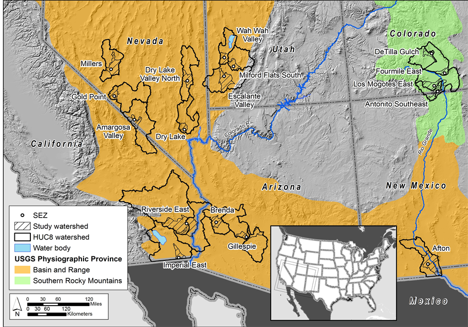
Figure 1. Physiographic settings of the 17 SEZ study watersheds in the six-state region of interest. Inset: Contiguous United States with extent rectangle.
climates with scarce surface waters and subtropical to tropical or desert vegetation [25] . The Southern Rocky Mountains province exhibits complex topography, including the highest peaks among those of the Rocky Mountains system of North America. Southern Rocky Mountains watersheds in this study have cool summers and very cold winters; vegetation includes coniferous forests and abundant surface waters [25] . The Colorado River and the Rio Grande lie in proximity to several of the study watersheds.
3. Methods
3.1. Data
Digital elevation model (DEM) and land cover datasets were used to develop an algorithm to identify the piedmont region where MFR occurs. The DEM layer consisted of seamless, gridded elevation data from the USGS National Elevation Dataset (NED) [26] at an approximately 10-m resolution, which represents average elevation over the land surface area of each pixel. The DEM layer was clipped to smaller rectangle areas around individual watersheds or clustered watershed groups to improve computational efficiency.
The California Gap Land Cover Mapping Project (CA-GAP) and the Southwestern Regional Gap Analysis Project (SWReGAP) datasets [27] [28] were used to extract land cover information at 30-m resolution. An elevation threshold was also applied using the DEM dataset for masking. The outputs from these procedures were overlain in order to determine the MFR zone within each watershed (Figure 2).
3.2. MFR Zone Delineation
Slope was first computed by using the DEM as the maximum change in elevation among the adjacent eight pixels at each location. Slope values were grouped into 100 classes through iterative self-organizing (ISO) classification [29] . ISO classification is a data clustering routine that identifies clusters of pixels based on natural

Figure 2. Workflow of the algorithm used to generate MFR zone maps.
groupings of cells with similar values through multiple iterations. The algorithm finalizes clusters when the number of cells that changes from one class to another becomes negligible. In the resultant ISO layer, a set of slope classes was selected as topographically consistent with the location of MFR based on the metric of pixel density. The pixel density metric was a measure based on the emergent patterns in the number of pixels classified into each class across the slope classes and was originally developed to examine the sensitivity of ephemeral stream channels to disturbances in arid environments [5] . In this study, a threshold value for pixel density was interactively set at 0.03 based on the approximate position of the density peak. The slope class corresponding to this threshold value (e.g., slope class = 5) and the nine subsequent classes (e.g., slope classes = 6 to 14) were identified as the piedmont region. The selected slope classes were qualitatively verified to coincide with MFR locations in the landscape through overlay analysis comparing the candidate MFR areas in the slope class data layer with alluvial fan features near each SEZ.
The slope class layer was converted into a binary layer that represented areas consistent with MFR (pixel value = 1) and those inconsistent with MFR (pixel value = 0). A 3- × 3-pixel maximum filter was applied to account for spatial autocorrelation within a local area across the watersheds. The resulting binary raster layer was converted to a polygon layer. Polygons with an MFR consistency value of 1 that were smaller than 50,000 m2 (<500 pixels) were reassigned to a value of 0 in order to compensate for artifacts from the data processing algorithm.
A land cover mask was created independently from the slope analysis to exclude irrelevant land cover types from further analysis. Developed land cover types were eliminated because they potentially limit or prevent groundwater recharge. Open water (water bodies and stream channels) was eliminated to map only areas of diffuse rather than focused recharge. Cultivated land cover types were eliminated because the net effect of agricultural irrigation on groundwater recharge depends on whether groundwater is pumped for irrigation, which the algorithm did not take into account. MFR-consistent polygons having one of these land cover types were reassigned to be MFR-inconsistent (value = 0). All other land cover types were identified as MFR-consistent (value = 1). An 11- × 11-pixel minimum filter was then applied to account for spatial autocorrelation within a local area across the study watersheds. This process accounted for the likely reduction in groundwater recharge occurring over fragmented versus continuous areas of MFR-consistent surfaces by removing small clusters of non-contiguous MFR-consistent areas. The data layer resulting from the land cover masking was converted to a polygon layer using the MFR consistency attribute (pixel values = 0 or 1) as the attribute value to create the polygons. Polygons with an MFR consistency value of 1 that were smaller than 10,000 m2 (<100 pixels) were reassigned to a value of 0.
The two polygon layers that resulted from the slope analysis and land cover masking were intersected to generate a single polygon layer. Areas with a value of 1 for both polygon layers (i.e., MFR-consistent polygons and no-mask polygons) were determined to be the final MFR candidate areas. The final MFR candidate areas were buffered by 100 m to account for a degree of uncertainty in the delineation of the MFR zone.
The output layer from the overlay analysis was clipped to the geographic area comprising elevations of the lower 50% of elevation range within each watershed. An elevation range layer was generated by binarizing the DEM data layer to reflect the upper and lower halves of elevation range (upper 50% of elevation range = 0 and lower 50% of elevation range = 1). This layer was converted to a polygon layer according to the binary elevation range attribute. The output layer from the MFR mapping algorithm was clipped to the topographic area with an elevation range value of 1, the lower 50% of elevation range. This step eliminated geoprocessing artifacts that were identified as belonging to the MFR zone but that were located at elevations above the mountain front.
3.3. Reliability Evaluation
In the absence of spatially explicit data that indicate MFR locations, the resulting MFR zone maps were qualitatively evaluated for their reliability using slope, surficial geology, soil, and land cover datasets. Distributions of slopes and surficial geologic types, and soils and land cover in the MFR zone maps were quantified and compared for consistency with the piedmont region, and consistency in promoting groundwater recharge, respectively.
MFR zone maps were overlain with the USGS Surficial Geology of the US map [30] . Relevant surficial geologic materials in this dataset included 1) alluvial sediments (i.e., clayto gravel-sized particles deposited by stream or sheetwash flow), 2) eolian sediments (i.e., siltto sand-sized particles deposited by wind), 3) lacustrine sediments (i.e., fineto coarse-sized particles deposited in perennial or ephemeral lakes of undrained basins), and 4) residual materials developed in carbonate, igneous, or sedimentary rock (i.e., particles resulting from the partial chemical dissolution of various types of bedrock rather than sediments that were transported).
MFR zone maps were also overlain with the US State Soil Geographic database published by the US Department of Agriculture, Natural Resources Conservation Service [31] to identify soil types captured in mapping results. Four hydrologic properties of soils were examined—drainage class, flood frequency, presence of ponding, and hydric classification. Drainage class indicated the relative ease of water infiltration. Ponding class indicated the potential for standing water in a closed depression, while flood frequency described the possibility for the temporary covering of the land surface by flowing water. Hydric class indicated soils under conditions of saturation long enough to develop anaerobic conditions in the upper layer. Soil hydrologic group was not analyzed for this study because this group is based on a calculation of infiltration rate from saturated hydraulic conductivity. Soil hydrologic group was not relevant for the purposes of this analysis because the soils in the arid watersheds examined did not develop under saturated conditions.
The slope data layer was intersected with the MFR zone maps to identify the spatial distribution of slope values throughout the mapped areas. The CA-GAP and SWReGAP land cover datasets were also intersected with the final maps to identify general land cover categories present in the mapped areas.
4. Results
The resulting maps showed that the MFR zones accounted for 40% of total watershed area studied (Table 2). The surface areas of the MFR zones were partially a function of watershed size and ranged across the 17 watersheds from 74 km2 (Four mile East) to 1547 km2 (Riverside East).The proportion of the MFR zone to total watershed surface area ranged from 13% (Four mile East) to 58% (Antonito Southeast). Mapped areas in most watersheds were generally clustered around the bases of mountainous features (e.g., Brenda MFR zone; Figure 3) and included areas with recognized overlying alluvial fan features near SEZs (e.g., Riverside East MFR zone; Figure 4). In a limited number of watersheds, however, the algorithm did not appear to delineate the MFR zone as reliably as in the majority of watersheds. In the Imperial East and Four mile East watersheds, the MFR zone appeared more dispersed in contrast to its typical location surrounding the bases of mountainous features. Portions of the mountain front in Four mile East were also not sufficiently represented in its MFR zone. A few such
Table 2 . Surface area and slope statistics of the MFR zone maps in the 17 study watersheds by physiographic provincea.
aVariance, standard deviation, and percentile values estimated from frequency data.
MFR locations in the basin floor can be seen in the Brenda MFR zone (Figure 3), but they are present to a lesser extent than in the Imperial East or Four mile East MFR zones. In addition, for the Wah Wah Valley, Milford Flats South, and Antonito Southeast watersheds, areas located outside the mountain front were included in the MFR zone delineation.
Reference data for slopes present in the MFR zones fell within a relatively narrow range in values specific to each MFR zone (Table 2). Median MFR zone slopes ranged from 0.9˚ (Imperial East) to 2.5˚ (Dry Lake), while slope values for the 90th percentile ranged from 3.3˚ (Four mile East) to 8.7˚ (Brenda). The maximum slope values in each MFR zone are much higher than slopes that would be found at the mountain front and likely do not represent real MFR locations in the landscape. However, the 90th percentile slope values were an order of magnitude lower than the corresponding maximum slope value found in each MFR zone, thus most slopes (i.e., >90%) present in the MFR zones were much lower than the maximum that was observed. The highly uncertain maximum values observed were therefore isolated instances. Some variability was seen in the results, with standard deviations that ranged from 1.4˚ (Four mile East) to 4.7˚ (Brenda and Dry Lake). MFR zone slopes showed little variation by physiographic province, with aggregated medians for MFR zone slope values that were comparable between those in the Southern Rocky Mountains and the Basin and Range provinces (i.e., 1.9˚ and
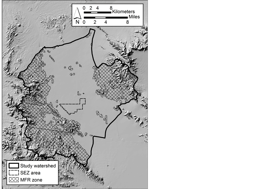
Figure 3. MFR zone for Brenda SEZ and study watershed.

Figure 4. Alluvial fan in Riverside East SEZ study watershed with MFR zone overlay. Inset: Riverside East SEZ and study watershed with extent rectangle.
1.8˚, respectively).
When slope was plotted against its percentage of area in each MFR zone, the shapes of slope distributions exhibited noticeable similarities among 13 of the 17 individual MFR zones (Figure 5). This characteristic distribution was typified by an asymmetrical, smooth curve skewed toward higher slope values that peaked between slopes of approximately 0.5˚ to 2.0˚. In this distribution, very flat areas (i.e., slopes near 0.0˚) accounted for only small percentages of total MFR zone surface area. This characteristic slope distribution was generally associated with MFR zones that were visually consistent with the previously discussed characteristics attributed to MFR locations, such as clustering around mountainous features and inclusion of overlying alluvial fan features.
Slope distributions for Imperial East, Four mile East, Wah Wah Valley, and Milford Flats South were notable exceptions to the similarities found among other MFR zone slope distributions (Figure 6). The single greatest percentage of MFR zone surface area was accounted for by 0.0˚ slopes in all four of these distributions. The Imperial East distribution also had a local peak at 0.3˚ slope, while Four mile East had three local peaks at slopes
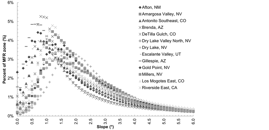
Figure 5. Distributions of slopes less than 6˚ for selected MFR zones as a percentage of MFR zone area (characteristic slope distribution).
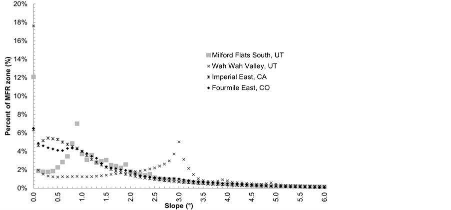
Figure 6. Distributions of slopes less than 6˚ for selected MFR zones as a percentage of MFR zone area (atypical slope distribution).
of approximately 0.8˚, 2.0˚, and 3.0˚ that successively decreased in the percentage of MFR zone area represented. In addition to the maximum percentages at 0.0˚ slope, the Wah Wah Valley and Milford Flats South distributions both lacked the smooth peak that was found in the characteristic distribution. These two distributions instead had sharp spikes in the percentage of MFR zone surface area at 3.0˚ and 0.9˚ slope values, respectively.
The overlay assessment using surficial geologic data indicated that alluvial, eolian, and lacustrine sediments, and discontinuous residual materials developed in carbonate, igneous, or sedimentary rock covered the MFR zones (Table 3). Thick alluvial sediments were the dominant surficial material overlying the MFR zones, covering 62% of total MFR zone surface area. In the Southern Rocky Mountains province, residual materials from igneous and metamorphic rocks were the dominant surficial materials associated with MFR zones. In the Basin and Range province, alluvial sediments were the primary constituent of MFR zones, in conjunction with residual materials that were present to a lesser extent.
The MFR zones were predominately covered with soils that were well drained or somewhat excessively drained (i.e., 95% of total MFR zone surface area), with little to no presence of ponding anywhere in the MFR zones. In addition, 98% of total MFR zone surface area indicated no potential for flooding. Finally, 92% of total MFR zone surface area had no hydric conditions (or was unclassified for hydric conditions).
The MFR zones were largely covered by shrub/scrub cover and grasslands/herbaceous cover (i.e., 61% and 20% of total MFR zone surface area, respectively; Table 4). Some barren lands were present (i.e., 13%). Regionally, shrub/scrub cover was more extensive in the Basin and Range MFR zones than in the Southern Rocky Mountains MFR zones (i.e., 72% and 4%, respectively). Grasslands/herbaceous cover was dominant in the Southern Rocky Mountains MFR zones (i.e., 83%).
5. Discussion
The MFR zones delineated by the algorithm were dominated by areas having slopes consistent with the piedmont region and overlain with arid grass or shrub communities growing on well-drained soils from alluvial sediments or residual geologic materials. The slope evaluation results suggested that the mapped areas were generally located at the mountain front as expected, apparent from the locations of MFR zones around the bases of mountainous features and overlying alluvial fan features that were present in MFR zones. Surficial geologic
Table 3 . Percentage of surficial geologic materials in MFR zones by physiographic province.
Table 4. Percentage of land cover types in MFR zone maps by physiographic province.
materials were also largely consistent with those at the mountain front. Soil hydrologic properties and vegetation in the MFR zones were consistent with conditions for which groundwater recharge would occur. The soil and land cover types that overlapped the MFR zones could promote groundwater recharge via moderate to high rates of water infiltration and limited evapotranspiration. These findings indicated that the algorithm generally performed well to reliably delineate locations of MFR in arid watersheds.
5.1. Slope
The slope percentile values and slope distributions found in the MFR zones indicated that slopes in the maps produced from this analysis agreed with the reference range for piedmont region slopes (0.5˚ - 11.3˚), which was determined based on field studies [32] -[34] and modeling work [14] . The 90th percentile slope values for all watersheds were well below 11.3˚, which means that more than 90% of slopes present in the MFR zone by area were below the maximum slope for the piedmont region from the literature. The shape of the curve in the characteristic slope distribution plot also showed that the majority of slope values occurred in the reference range for the piedmont region and that only comparatively small percentages of MFR zone surface area were accounted for by slopes outside this range (<0.5˚ or >11.3˚). Calculated from the slope distributions, 88.5% of total MFR zone surface area was found to have slopes within this reference slope range for the piedmont region. This suggested that the algorithm reliably detected MFR zones in most watersheds according to the conceptual definition of the MFR zone introduced by Wilson and Guan [16] .
The MFR zones having atypical slope distributions provided important examples of the effect of topographic variation on reliable delineation of the MFR zones. These MFR zones contained considerably different topography from that considered typical of the Basin and Range province. The typical topography associated with mountain systems of the Basin and Range province is characterized by north-south-oriented, faulted mountains surrounding a flat, arid valley. Small hill or dune features in the basin floors of the Imperial East and Four mile East watersheds led to the dispersed, highly uncertain MFR zone detections in the basin floor outside of the mountain front. In Imperial East particularly, the large, migrating Imperial Sand Dunes field visibly affected the analysis in this watershed. These results suggested that the algorithm might be better suited for delineating MFR zones in settings that exhibit characteristic Basin and Range topography with relatively flat basin floors than in settings that lack these conditions.
Unreliable delineation of the MFR zone also possibly resulted from improper selection of the slope classes composing the MFR zone, a function of the single pixel density threshold, 0.03, that was used in zone delineation in all watersheds. The topography in the Wah Wah Valley and Milford Flats South watersheds appears to conform to characteristic Basin and Range topography where the algorithm is thought to perform well; yet their MFR zones and slope distribution plots demonstrated atypical results. The largest percentage area was accounted for by 0.0˚ slopes in their MFR zones, which indicated that large extents of the basin floor were captured in the mapping results. In addition, the Wah Wah Valley and Milford Flats South slope distribution plots demonstrated spikes rather than the smooth peak that was associated with most other MFR zones. Further investigation is warranted to more conclusively determine whether the pixel density threshold affected MFR zone delineation in the Wah Wah Valley and Milford Flats South watersheds or whether topographic variation was a factor that affected the analysis. If the pixel density threshold was a factor, then calibration of the pixel density threshold to individual watersheds could improve the reliability of zone delineation.
Patterns corresponding to differences between physiographic provinces were expected in the slope distributions of the MFR zones because variability was observed among the pixel density plots for the Southern Rocky Mountains watersheds during algorithm development [5] . The pixel density threshold value, 0.03, guided selection of the 10MFR slope classes that were used to identify candidate MFR locations. This value was interactively chosen because it corresponded to an observed peak in pixel density that was interpreted as the valley edge of the piedmont slope. Unlike for the Basin and Range study watersheds, a plateau rather than a peak corresponded to this value for the Southern Rocky Mountains study watersheds. This plateau was interpreted to represent greater topographic variation on the valley floors of the Southern Rocky Mountains study watersheds than on those of the Basin and Range study watersheds. However, variability in the slopes of mapped MFR zones was not limited to the Southern Rocky Mountains province as expected. Two of three Utah MFR zones and one California MFR zone in the Basin and Range province indicated atypical slope distributions, compared with one of four Southern Rocky Mountains MFR zones. Slope distributions were overall relatively similar between the two provinces. Therefore, topographic variation in the study watersheds was an important factor affecting the reliability of MFR zone delineation by the algorithm, but one that was not limited to the Southern Rocky Mountains province in this analysis.
5.2. Geology
Overall, the surficial geologic materials present in the MFR zone maps were consistent with those expected at the mountain front. Characteristics of geologic materials found within the MFR zones supported reliability in MFR zone delineation. MFR zones were largely covered by alluvial sediments (i.e., 62% of total MFR zone area; Table 3), which is consistent with the depositional setting at the mountain front where water and sediment are received from higher elevations. Although alluvial sediments are also the predominant material that covers the valley floor in most watersheds, the slope distributions within most MFR zones showed only comparatively small percentages of MFR zone area composed by slopes below the reference minimum slope for the piedmont region (i.e., <0.5˚). Because alluvial sediments were more extensive than areas with basin floor slopes, most areas that were overlapped by alluvial sediments were also consistent with a location in the piedmont region.
Residual materials that were developed from bedrock through chemical dissolution or physical disintegration were also present in the MFR zones. The mountain front is a transition zone between two different topographic regions—the mountain face and the valley bottom [16] . Thus, this region could contain surficial geologic materials common to both settings. While alluvial sediments are associated with the depositional setting at the mountain front, thin soils overlie bedrock on the mountain face and would be consistent with the presence of residual materials in the MFR zones. Composition of geologic materials overlying the MFR zone maps also reflected local conditions. For example, eolian deposits (e.g., dune sands) were present in the MFR zones of desert watersheds, including Afton and Imperial East.
5.3. Soil
Overall, the soil hydrologic properties dominant in the MFR zones supported the reliability of locations delineated by the algorithm. The MFR zones were overlain by soils that were associated with moderate to high rates of water infiltration, which would support the potential for groundwater recharge. Groundwater recharge is generally greater in soils that have higher hydraulic conductivity than soils that have lower hydraulic conductivity. Higher hydraulic conductivity allows water to infiltrate more easily and results in soils that are more well drained [1] [35] . Most of the MFR zone surface area was dominated by well-drained soils that implied moderate to high rates of water infiltration that would support groundwater recharge. Like drainage class, the ponding, flooding, and hydric characteristics for the MFR zones were consistent with soils having moderate to high infiltration rates because they indicated no standing water, little to no possibility of flooding, and few locations with hydric conditions. In contrast, areas with lower rates of water infiltration would generally be associated with more extensive poor drainage, standing water, flooding, and hydric conditions.
5.4. Land Cover
Land cover types associated with the MFR zones consisted of vegetation that would support moderate to high rates of groundwater recharge in desert regions. In arid climates, the presence of vegetation can increase infiltration capacity by protecting soil stability and creating habitat for soil biologic communities that affect water balance [36] . In general, higher groundwater recharge rates are associated with annual crops and grasses compared with trees and shrubs because of the relatively shorter growing season and shallower root depth of the former, resulting in a lower degree of water loss from the system through evapotranspiration [37] [38] . The most extensive land cover types in the MFR zones were scrub/shrub cover and grasslands/herbaceous cover, both of which would support higher rates of groundwater recharge. While shrub/scrub cover leads to some evapotranspiration, the presence of vegetation in general encourages infiltration by protecting soil stability. Therefore, the evaluation results for overlying land cover types generally supported the interpretation that the algorithm reliably delineated areas promoting groundwater recharge.
The land cover types dominant in the MFR zones varied by local conditions within physiographic provinces; they did not vary, however, in terms of implications for infiltration rates. The largest percentage of land cover in MFR zones in both the Basin and Range and Southern Rocky Mountains provinces was either grasslands/herbaceous cover or shrub/scrub cover, both of which are consistent with moderate rates of water infiltration as discussed previously. Forest cover that could limit groundwater recharge through increased evapotranspiration was present but accounted for less than 5% of total MFR zone surface area. Similarly, wetlands, which could indicate limited water infiltration of soils, were also present but accounted for less than 2% of total MFR zone surface area. The MFR zone maps in both provinces also included negligible areas of land cover types specifically excluded during land cover masking (e.g., disturbed, developed, and agricultural lands). These land cover types were inadvertently included in the final MFR zone maps from the overlay analysis stage of the algorithm when the maps were buffered by 100 m to account for uncertainty in zone delineation.
6. Summary
In this study, a method was developed to map MFR locations based on slope and land cover types in arid, mountainous watersheds of the western United States. Reliably delineating the spatial distribution of MFR is valuable for allowing researchers to quantify aspects of the hydrologic processes associated with these areas and for helping local managers to consider protection of critical groundwater recharge regions when making land development decisions. The algorithm developed in this study is a novel approach for delineating MFR locations that integrates a terrain analysis approach with land cover that accounts for groundwater recharge rates.
This algorithm produced maps of spatial MFR distribution in 17 arid study watersheds. Rigorous multi-source qualitative assessment (e.g., visual inspection and overlay analysis) was performed using datasets of slope, surficial geologic materials, soils, and land cover types to examine the reliability of the MFR zone delineation and account for the lack of reference data for the geographic distribution of MFR locations. The multi-source assessment indicated that MFR zones were generally located in the piedmont region of each watershed and exhibited a strong association with desert grasslands or shrub cover growing in well-drained soils from alluvial sediments or residual materials. The location of MFR zones primarily in the piedmont region based on associated slopes and surficial geologic materials was consistent with their presence at the mountain front. The soil and land cover types indicated conditions that could promote groundwater recharge via moderate to high water infiltration rates and limited evapotranspiration. All of these factors supported the reliability of the algorithm for identifying MFR locations in most of the watersheds examined.
Applicability of the method, however, was limited to particular topographic conditions. The algorithm appeared to be best suited for watersheds that exhibited the characteristic topography associated with mountain systems of the Basin and Range Physiographic Province. Topographic variation on the basin floor affected the reliability with which the algorithm identified the piedmont region using slope.
The refinement of the algorithm could include improved screening, calibration, and validation methods to improve the reliability of MFR zone delineation. Watersheds could be screened for topographic consistency with Basin and Range characteristics to assess the suitability of applying the algorithm and to determine whether the results would be meaningful. In addition, the pixel density threshold value used to select MFR-consistent slope classes in the slope analysis step of the algorithm could be calibrated to the individual watersheds or regions where the method is being applied, rather than utilizing the single value that was used for all watersheds in this analysis. Finally, robust, quantitative validation of results could be accomplished through the collection of field data to map locations of MFR in the watersheds studied. This field data would provide reference datasets with which to compare algorithm results and assess their accuracy quantitatively.
Acknowledgments
The authors thank Heidi M. Hartmann for insightful comments on the manuscript. The submitted manuscript has been created by UChicago Argonne, LLC, Operator of Argonne National Laboratory (“Argonne”). Argonne, a US Department of Energy (DOE) Office of Science laboratory, is operated under Contract No. DE-AC02- 06CH11357. The US Government retains for itself, and others acting on its behalf, a paid-up nonexclusive, irrevocable worldwide license in said article to reproduce, prepare derivative works, distribute copies to the public, and perform publicly and display publicly, by or on behalf of the Government. Funding for this project was supported by the US Department of the Interior-Bureau of Land Management under interagency agreement, through US Department of Energy contract DE-AC02-06CH11357.
References
- Keese, K.E., Scanlon, B.R. and Reedy, R.C. (2005) Assessing Controls on Diffuse Groundwater Recharge Using Unsaturated Flow Modeling. Water Resources Research, 41. http://dx.doi.org/10.1029/2004WR003841
- Stonestrom, D.A. and Harrill, J.R. (2007) Chapter A—Climatic and Geologic Framework. In: Stonestrom, D.A., Ed., Ground-Water Recharge in the Arid and Semiarid Southwestern United States, US Geological Survey, Reston.
- Copeland, H.E., Pocewicz, A. and Kiesecker, J.M. (2011) Geography of Energy Development in Western North America: Potential Impacts on Terrestrial Ecosystems. In: Naugle, D.E., Ed., Energy Development and Wildlife Conservation in Western North America, Island Press, Washington DC.
- Leu, M., Hanser, S.E. and Knick, S.T. (2008) The Human Footprint in the West: A Large-Scale Analysis of Anthropogenic Impacts. Ecological Applications, 18, 1119-1139. http://dx.doi.org/10.1890/07-0480.1
- US Bureau of Land Management and US Department of Energy (2012) Final Programmatic Environmental Impact Statement (PEIS) for Solar Energy Development in Six Southwestern States. Bureau of Land Management and US Department of Energy, Bureau of Land Management, Washington DC.
- Aishlin, P. and McNamara, J.P. (2011) Bedrock Infiltration and Mountain Block Recharge Accounting Using Chloride Mass Balance. Hydrological Processes, 25, 1934-1948. http://dx.doi.org/10.1002/hyp.7950
- Covino, T.P. and McGlynn, B.L. (2007) Stream Gains and Losses across a Mountain-to-Valley Transition: Impacts on Watershed Hydrology and Stream Water Chemistry. Water Resources Research, 43. http://dx.doi.org/10.1029/2006WR005544
- Manning, A. and Solomon, D. (2003) Using Noble Gases to Investigate Mountain-Front Recharge. Journal of Hydrology, 275, 194-207. http://dx.doi.org/10.1016/S0022-1694(03)00043-X
- Scanlon, B.R., Keese, K.E., Flint, A.L., Flint, L.E., Gaye, C.B., Edmunds, W.M. and Simmers, I. (2006) Global Synthesis of Groundwater Recharge in Semiarid and Arid Regions. Hydrological Processes, 20, 3335-3370. http://dx.doi.org/10.1002/hyp.6335
- Grimm, N.B., Chacon, A., Dahm, C.N., Hostetler, S.W., Lind, O.T., Starkweather, P.L. and Wurtsbaugh, W.W. (1997) Sensitivity of Aquatic Ecosystems to Climatic and Anthropogenic Changes: The Basin and Range, American Southwest and Mexico. Hydrological Processes, 11, 1023-1041. http://dx.doi.org/10.1002/(SICI)1099-1085(19970630)11:8<1023::AID-HYP516>3.0.CO;2-A
- Welch, L.A. and Allen, D.M. (2012) Consistency of Groundwater Flow Patterns in Mountainous Topography: Implications for Valley Bottom Water Replenishment and for Defining Groundwater Flow Boundaries. Water Resources Research, 48. http://dx.doi.org/10.1029/2011WR010901
- Burness, S., Chermak, J. and Brookshire, D. (2004) Water Management in a Mountain Front Recharge Aquifer. Water Resources Research, 40. http://dx.doi.org/10.1029/2003WR002160
- Hashimoto, A., Oguchi, T., Hayakawa, Y., Lin, Z., Saito, K. and Wasklewicz, T.A. (2008) GIS Analysis of Depositional Slope Change at Alluvial-Fan Toes in Japan and the American Southwest. Geomorphology, 100, 120-130. http://dx.doi.org/10.1016/j.geomorph.2007.10.027
- Strudley, M.W. and Murray, A.B. (2007) Sensitivity Analysis of Pediment Development through Numerical Simulation and Selected Geospatial Query. Geomorphology, 88, 329-351. http://dx.doi.org/10.1016/j.geomorph.2006.12.008
- Volker, H.X., Wasklewicz, T.A. and Ellis, M.A. (2007) A Topographic Fingerprint to Distinguish Alluvial Fan Formative Processes. Geomorphology, 88, 34-45. http://dx.doi.org/10.1016/j.geomorph.2006.10.008
- Wilson, J.L. and Guan, H. (2004) Mountain-Block Hydrology and Mountain-Front Recharge. In: Hogan, J.F., Phillips, F.M. and Scanlon, B.R., Eds., Groundwater Recharge in a Desert Environment: The Southwestern United States, American Geophysical Union, Washington DC, 294. http://dx.doi.org/10.1029/009WSA08
- Bedrossian, T.L., Roffers, P., Hayhurst, C.A., Lancaster, J.T. and Short, W.R. (2012) Geologic Compilation of Quaternary Surficial Deposits in Southern California (Special Report 217). Department of Conservation, California Geological Survey, Sacramento.
- Brown, D.G., Lusch, D.P. and Duda, K.A. (1998) Supervised Classification of Types of Glaciated Landscapes Using Digital Elevation Data. Geomorphology, 21, 233-250. http://dx.doi.org/10.1016/S0169-555X(97)00063-9
- Dragut, L. and Blaschke, T. (2006) Automated Classification of Landform Elements Using Object-Based Image Analysis. Geomorphology, 81, 330-344. http://dx.doi.org/10.1016/j.geomorph.2006.04.013
- Manis, G., Lowry, J. and Ramsey, D.R. (2001) Preclassification: An Ecologically Predictive Landform Model. US Geological Survey. GAP Analysis Bulletin, 10.
- Prima, O.D.A., Echigo, A., Yokoyama, R. and Yoshida, T. (2006) Supervised Landform Classification of Northeast Honshu from DEM-Derived Thematic Maps. Geomorphology, 78, 373-386. http://dx.doi.org/10.1016/j.geomorph.2006.02.005
- Saadat, H., Bonnell, R., Sharifi, F., Mehuys, G., Namdar, M. and Ale-Ebrahim, S. (2008) Landform Classification from a Digital Elevation Model and Satellite Imagery. Geomorphology, 100, 453-464. http://dx.doi.org/10.1016/j.geomorph.2008.01.011
- Singh, V. and Tandon, S.K. (2010) Integrated Analysis of Structures and Landforms of an Intermontane Longitudinal Valley (Pinjaur Dun) and Its Associated Mountain Fronts in the NW Himalaya. Geomorphology, 114, 573-589. http://dx.doi.org/10.1016/j.geomorph.2009.09.019
- Graf, W.L. and Geological Society of America (1987) Geomorphic Systems of North America. Geological Society of America, Boulder.
- Wiken, E., Nava, F.J. and Griffith, G. (2011) North American Terrestrial Ecoregions—Level III. Commission for Environmental Cooperation, Montreal.
- US Geological Survey (2012) National Elevation Dataset. http://ned.usgs.gov/index.html
- Lennartz, S., et al. (2008) Final Report on Land Cover Mapping Methods for California Map Zones 3, 4, 5, 6, 12, and 13. 30 p.
- Lowry Jr., J.H., Ramsey, R.D., Boykin, K., Bradford, D., Comer, P., Falzarano, S. and Wolk, B. (2005) The Southwest Regional Gap Analysis Project Final Report on Land Cover Mapping Methods. Utah State University, Logan.
- Tou, J.T. and Gonzalez, R.C. (1974) Pattern Recognition Principles. Addison-Wesley Publishing Company, 377 p.
- Soller, D.R., Reheis, M.C., Garrity, C.P. and Van Sistine, D.R. (2009) Map Database for Surficial Materials in the Conterminous United States. Data Series, US Geological Survey, Reston.
- US Department of Agriculture Natural Resources Conservation Service (2012) State Soil Survey Geographic Database. http://www.nrcs.usda.gov/wps/portal/nrcs/main/soils/survey/geo/
- Dohrenwend, J.C. and Parsons, A.J. (2009) Pediments in Arid Environments. In: Abrahams, A.D. and Parsons, A.J., Eds., Geomorphology of Desert Environments, 2nd Edition, Springer, New York, 377-411. http://dx.doi.org/10.1007/978-1-4020-5719-9_13
- Peterson, F.F. (1981) Landforms of the Basin and Range Province Defined for Soil Survey. Technical Bulletin 28, Nevada Agricultural Experiment Station, Max C. Fleischmann College of Agriculture, University of Nevada Reno, Reno, 56.
- Blissenbach, E. (1954) Geology of Alluvial Fans in Semiarid Regions. Geological Society of America Bulletin, 65, 175. http://dx.doi.org/10.1130/0016-7606(1954)65[175:GOAFIS]2.0.CO;2
- Nolan, B.T., Baehr, A.L. and Kauffman, L.J. (2003) Spatial Variability of Groundwater Recharge and Its Effect on Shallow Groundwater Quality in Southern New Jersey. Vadose Zone Journal, 2, 677-691. http://dx.doi.org/10.2136/vzj2003.6770
- Thompson, S.E., Harman, C.J., Heine, P. and Katul, G.G. (2010) Vegetation-Infiltration Relationships across Climatic and Soil Type Gradients. Journal of Geophysical Research: Biogeosciences, 115. http://dx.doi.org/10.1029/2009JG001134
- Havstad, K.M., Peters, D.P.C., Skaggs, R., Brown, J., Bestelmeyer, B., Fredrickson, E. and Wright, J. (2007) Ecological Services to and from Rangelands of the United States. Ecological Economics, 64, 261-268. http://dx.doi.org/10.1016/j.ecolecon.2007.08.005
- Western Regional Climate Center (2012) Western U.S. Climate Historical Summaries, Climatological Data Summaries (LCD), Selected Stations. http://www.wrcc.dri.edu/Climsum.html
NOTES

*Corresponding author.

1This analysis included SEZs that were assessed in the Solar PEIS; two additional SEZs (Agua Caliente SEZ in Arizona and West Chocolate Mountains SEZ in California) have been identified to date.