iBusiness
Vol.3 No.3(2011), Article ID:7473,14 pages DOI:10.4236/ib.2011.33033
Finance and Centre-Periphery Dynamics: A Model
![]()
University of Salento, Lecce, Italy.
Email: apaolilli@alice.it
Received May 2nd, 2011; revised July 3rd, 2011; accepted July 15th, 2011.
Keywords: Finance, Centre-periphery dynamics
ABSTRACT
In the last few decades we have witnessed a marked process of economic globalization (that is the growing interrelation and integration of the economic systems of the whole world), accompanied and favoured by what is called financialization (whose definition is more problematic, but we can identify it as the growing relative importance of financial profits compared to those deriving from trade and production of real goods). In this paper, after briefly discussing and defining the two phenomena in the light of the debate about them, we will present a mathematical model to study their effects on the economic development of regions with a different initial capital set-up, which includes human and organizational capital. The model shows that low wages in certain conditions can determine high interest rates, favouring financial flows from peripheral areas to developed countries.
1. Introduction
The role of finance in economic development has been the focus of widespread discussion1. The connection between economic development and the reduction of poverty has been at the centre of a heated debate. The work of Lopez [1] identifies at least two branches of the literature which furnish a quite different response to the question of the relation between development and poverty reduction2.
On the question of the relation between finance and development it is not clear which comes first. There is most likely a wash back effect, although, according to studies by Calderon and Liu [2], the effects of financial growth on economic growth are stronger than those of the latter on the former and they are also more pronounced in developing economies than in developed ones.
Financial growth may be hampered by low interest rates which may discourage saving and thus make investments sub-optimal. The low cost of money might also encourage not very efficient investments. In this regard, McKinnon [5] and Shaw [6] have independently found that most of the state’s negative impact comes from the imposition of artificially low interest rates.
The recommendation was therefore to leave as much freedom as possible for the unfolding of economic forces. This recommendation, on the other hand, was in line with the general climate of those years, during which many scholars began to believe that state intervention in the economy was the main obstacle to achieving prosperity.
The world economy has therefore abandoned “financial repression”, and globalization has been increasingly characterized and accelerated by what is called “financialization”. The result, however, has been far beyond expectations: interest rates raised more and for longer than expected, especially in less developed countries [7]. This resulted in strangulation of small and medium-sized enterprises, which have no easy access to direct financing, and in a compression of wage levels.
There is still no common agreement about the exact meaning of the term “financialization”. Krippner [8] provides a discussion on the meaning assigned to it by various scholars who have an interest in this phenomenon:
• Growth of equity values as a form of “corporate governance”;
• Growing dominion of systems based on the financial markets rather than on “bank intermediation”;
• The increase of economic and political power of the “rentier class”;
• Explosion of financial intermediation caused by the increasing number of technical tools.
Krippner, for her part, in identifying the phenomenon underlines the growing relative importance of financial profits compared to those deriving from trade and the production of real goods.
Epstein [9] maintains that each of these definitions captures a particular aspect of the “financialization” phenomenon and adds that, in a nutshell, it is the growth of the financial institutions, markets, actors and motivations in National and International economic operations.
Also in the viewpoint of Palley [10] financialization is a process “whereby financial markets, financial institutions, and financial elites gain greater influence over economic policy and economic outcomes” [10] and therefore it is essentially an abnormal growth of finance, if compared to production activities.
In Palley’s opinion, as well as a growing importance of the financial sector over the real one, and a resulting transfer of resources for the benefit of the former, financialization has also caused an increasing inequality in income distribution and a stagnation of wages [10] and it has transformed the functioning of economic systems at both micro and macro-economic levels. At the macro level it is supposedly associated with the slowdown in growth and a greater fragility of the financial systems [10], as shown by the recurrent crises [11]. On the other hand, these crises have a less and less localized dynamic. Investments are made far from the places where the savings originate, according to a short-term logic, focused on getting quick returns. These phenomena may seem new and quite typical of our times, and this is certainly true if we look at their size and their spatial and temporal aspects, but actually they are not without historical precedent. Andriani [11] notes that the current process of globalization and financialization is not new and irreversible, because it has at least a historical precedent (of which, however, the scholar emphasizes the differences, in the period from the second half of 1929 [11]3.
2. Modelling Financialization
Before building a model to describe financialization, we must identify the essential dynamics of this phenomenon. In fact we must represent these dynamics with the utmost simplicity consistent with the need not to lose relevant information.
Andriani notes that the financialization process emanates from the real economy and then feeds back onto it [14]. The origin of development, in fact, is determined by an accumulation process. This can be started simply by saving, resulting in its turn from a surplus production or, following Schumpeter [15], by the creation on the part of the banking system, of means of payment, which become available for investment of innovative entrepreneurs who remove them from consumption.
Whichever way it began, the accumulation process, once started in an area (which we will call A), tends to expand into other areas if they are able to offer access to natural and human resources, or for selling products so as to ensure further growth of capital. We will call these expansion areas B. The greater profitability can be determined essentially by two factors: lower costs (for equal productivity) or higher revenues. The latter may result from various causes, among which, however, there is a higher productivity due to a relative abundance of some factors.
The investment in B implies an increase in local revenues, but only for the salary component, with a consequent low local saving. The savings generated may also not necessarily involve investment in B by local entrepreneurs, because the local banking system may prefer financing activities already underway, even if they are of foreign origin. All this can then make economy B into a satellite of A. Obviously this process is more likely and more rapid when the financial means allowing a relocation of investment are more flexible. In addition, the ability to quickly move capital gives landowners a greater power over employees, who are therefore forced, for the same productivity, to accept lower wages. This happens even in the country where accumulation started, thus prefiguring a polarization that is not only territorial but also functional (between the different components of the economic system).
In the following sections we will try to transfer into a mathematical model the dynamics we have just described, simplifying them as far as possible, but saving those which are essential for meaningful results to be obtained.
3. Mathematical Model
The model we are presenting at first will referred to a single closed and homogeneous economic system. We assume, for the sake of simplicity, that the only cost for entrepreneurs, besides the interest rate, is wages, and that prices are stable. Productivity, moreover, depends on the difference between the target wage T and the real wage w. T could be identified with the real wage received by workers in central areas or even with an amount considered reasonable in relation to productivity. The closer the workers’ wage is to T, the greater their effort and therefore their productivity4.
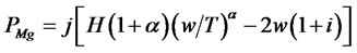
The number of workers who offer their labour will depend on the wages (in fact we can suppose that, if the wage is too low, workers will move to other regions). The equation of profit (net of interest on financing) will be:
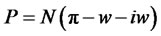 (3.1)
(3.1)
As a result of the arguments above, we can write the function of productivity:
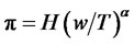 (3.2)
(3.2)
Naturally we assume w ≤ T and also α < 1 (to make the model able to exhibit decreasing marginal outputs). The first hypothesis (w ≤ T) implies that the maximum effort is produced with a wage equal to target T and that beyond this limit the effort cannot grow, because it is already at its maximum value.
If w = T, we have π = H H, then, is the maximum production of a worker in a given environment. Its value, in fact, is not unrelated to the geographical location of the firms. If the location is peripheral (i.e. if markets and/or supply sources are distant), the transport costs will reduce profits by acting on H. In fact the production will be lower if a portion of the investment is channelled into transport rather than into direct production. On the other hand H can vary from place to place, not only due to the distance (between markets or between factors), but also because of more complex reasons such as the presence (or absence) of agglomeration economies, human capital and (above all) organizational capital (not easily transferable).
Also N, the number of workers which offer their labour, as mentioned above, depends on w. For the sake of simplicity we can assume that the relation between N and w is linear:
 (3.3)
(3.3)
Inserting 3.2 and 3.3 in 3.1, we obtain:
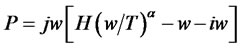 (3.4)
(3.4)
Equalizing to 0 the first derivative of 3.4, with respect to w, we can find the conditions which maximize profit:
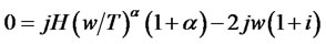 (3.5)
(3.5)
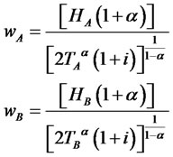
The wage which maximizes profit (which we will call w*: calculations in fn5) is:
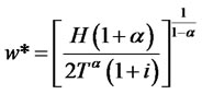 (3.6)
(3.6)
This wage can be, in dependence of the values of the parameters H, α, T and i (j is irrelevant) less than, equal to or greater than T. However we have assumed that the effort is maximum when w = T and therefore w* will never exceed T.
However we can easily see, by examining 3.6, that the equilibrium wage grows when productivity (expressed by H) increases, and that it is suffers a negative effect not only from the interest rate i (Figure 1 shows how an increase in i, not improbable in zones which, being depressed, have a higher risk of failures, reduces w*), but from the target wage T. This is due to the fact that a higher target, for any given wage less than w*, causes a less intense effort.
Notice, incidentally, that w* can be equal to T only if
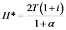 (3.7)6
The value of H (i.e. H*) which guarantees an optimal wage (for the entrepreneurs) and allows the last to equalize the target T (we could suppose that this condition can happen in the central areas) grows, therefore, if the target T and the interest rate i increase and decrease if α grows. From 3.7 we can obtain the value of T compatible with a certain productivity H (i.e. T*, which allows equality between w* and T*):
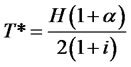 (3.8)
(3.8)
3.8 shows that an increase of the interest rate reduces T*, i.e. the wage to which workers can realistically aspire.
We have underlined that H in a peripheral region is usually lower than in a central area.
We could ask what happens in a similar circumstance. As we can see by examining 3.4, it is not only the equilibrium wage w*, but also the profit that decreases when H is reduced. To check what happens when two regions, a central one (which we will name A) and a peripheral (B), with HA > HB, interact, we have to compare the
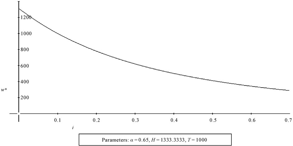
Figure 1. The graph shows the relation between the interest rate i (independent variable) and the equilibrium wage w*.
marginal profits of the two regions and not the average profits7 For this purpose, then, it will be useful to use the following relation, which is the first derivative, with respect to w, of the profit:
 (3.9)
(3.9)
At this point, however, it is also necessary to distinguish at least two types of peripheral areas: those with the same target wage as the central area and those with a lower target. In fact the peripheral regions which are next to the central area8, with no geographical, political or linguistic and cultural barriers, will show, more probably than other more distant or less integrated regions, a target wage closer to the wages received by the workers of the central area.
We have already seen that a reduction of H reduces w*. We must add that in this case also the supply N, which depends on w, decreases.
Generally if HA > HB there will be a flow of capital from B to A (i.e. towards the centre) because, if TA = TB, the profits are greater in A, and this will happen with greater intensity if iA < iB.
However the opposite phenomenon is also possible, i.e. the flow of financial resources towards the peripheral areas. This will happen above all if the target of the workers in the latter areas is lower than that of the workers in the central areas (TA > TB), making them work harder for the same wage.
To make a comparison, we must use two relations as 3.9, one referring to the central area A, the other to B. In this way we will able to know the direction of investments and also to what extent they will be active:
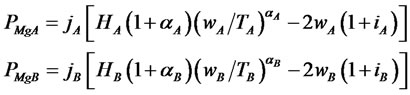 (3.10)
Due to the fact that the parameter j is irrelevant in the determination of w*, we will assume in all cases jA = jB. We will assume, moreover, the following condition (A being the central zone): HB < HA. As for interest rates, although it is reasonable to assume that they are usually but not necessarily higher in the peripheral zones, we will assume their equivalence, i.e. iA = iB, while for TB we will consider both the possible hypotheses, i.e. both TB = TA, and TB < TA. If TB is lower than TA, it is possible that lower wages are not associated to a lower effort, and this could attract investments from area A and hinder disinvestment by local firms (despite the lower value of HB).
To verify these hypotheses, it is useful to insert 3.10 into a system of differential equations:
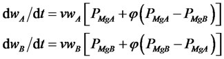 (3.11)9
In these equations v is an investment variation coefficient. For the sake of simplicity, we can assume that it has the same value in the two areas (vA = vB = v). We assume that also φ, which measures the degree of openness of the two economic systems towards each other, has the same value in the two areas.
By observing 3.11 we can see that if the marginal profit in A is greater than in B, wages and investments will grow in A and will decrease in B, and vice versa. The second term of 3.11 in fact describes a variation in the capital invested in the respective areas which proportional to the marginal profits and also to the difference (if positive) between these marginal profits, wages and employment in the area under consideration.
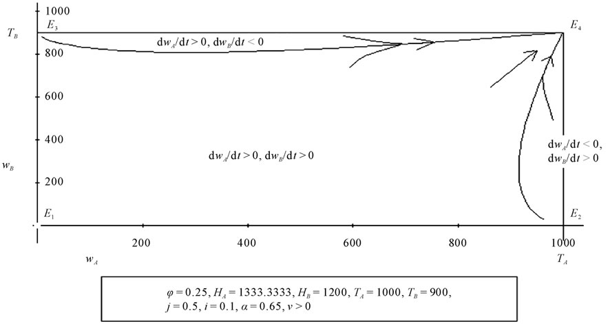
Figures 2(a), (b), 3, 6, and 7 show the values of wA
 (a)
(a)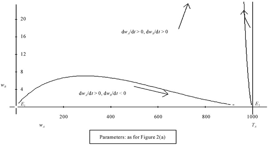 (b)
(b)
Figure 2. (a) The graph shows the combinations of wA and wB which may or may not imply, for given values of the parameters (shown in the bottom of the figure), a growth of wages (and profits) in areas A and B; (b) The figure shows a detail of the graph of Figure 2(a), evidencing how, near the axis of abscissas, there are combinations of the wA and wB for which wB decreases (we have an analogous situation near the axis of ordinates, where wB grows and wA decreases).
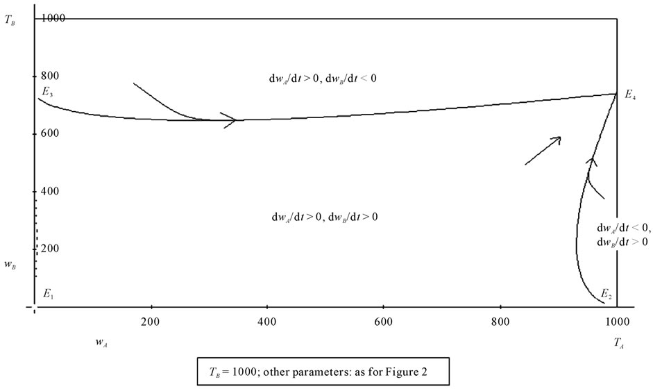
Figure 3. The graph shows how the equilibrium wage of the area B (in E4) is lower than in Figure 1, in dependence of a higher value of TB (1000 instead of 900).
and wB, whether or not they are associated to a growth in the respective areas, ceteris paribus, for different values of φ, TA, TB. The equilibrium points are E1, E2, E3 and E4. The first is a trivial point, because it entails the absence of investments and economic activities in both regions, E2 entails the absence of investments in area B, E3 the absence of investments in area A. E4 is the only stable equilibrium point, implying an effective equilibrium between the two regions, and therefore we will concentrate on it.
The coordinates of E4 are the following10:
 (3.12)
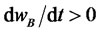
We have already shown when examining 3.6 that the growth of T reduces the equilibrium wage. Therefore, if TB is related to the wage of the central area (A), since we can assume that the latter is incompatible with the productivity of the peripheral area for the purpose of profit maximization, the equilibrium wage of the peripheral zone will decrease (see Figure 3). This is confirmed by the numerical simulations of Figures 4 and 5, in which the sole parameter that changes value is, precisely, TB (900 in the simulation of Figure 4, 1000 in the simulation Figure 5): the final wage wB in the second case is far lower.
The growth of φ, on the other hand, does not affect the final equilibrium. Figure 6, in fact, shows that, even when sets of values of wA and wB associated to their growth are changed, E4 does not change. However the area of combinations of wA and wB which cause a growth of both the variables ( and
and ) decreases.
Generally, however, high values of φ (which imply a great sensitivity of investments to the difference in profitability between the two areas) cause a delay in reaching the equilibrium. In addition, if the value of wA is quite a bit higher than the value of wB (showing a significant difference between the development of the two areas), before moving towards the final equilibrium value it can greatly decrease (see Figure 6: evolutionary trajectories in the zone ,
, ).
).
Figure 7 shows a situation in which the propensity to relocation is very high (φ = 11): the area of combinations of wA and wB which cause both of them to grow is divided into two zones separated by the combinations which bring about the growth of wA alone. This is indicative of the fact that if two economic systems, with dif-
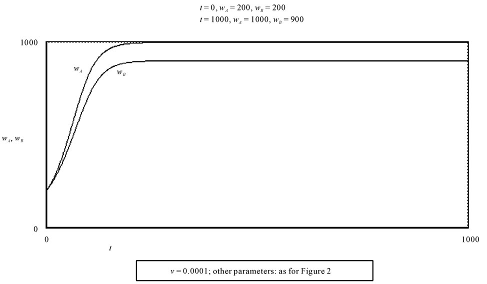
Figure 411. The numerical simulation presented in the diagram shows the evolution of wA and wB, for given values of the parameters. The value of wB, in particular, is 900.
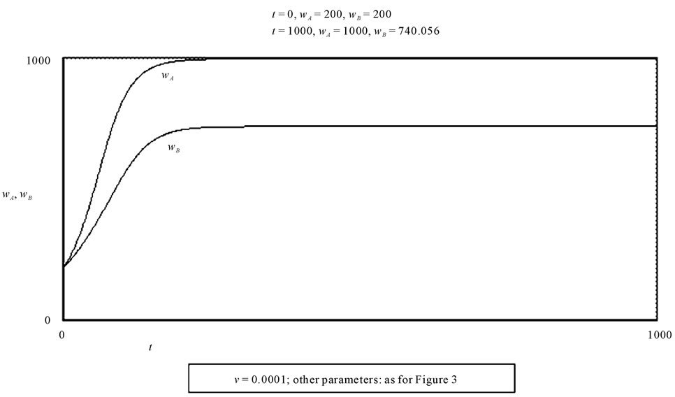
Figure 5. The graph shows a numerical simulation like that of Figure 4, but with a higher value for the target TB (1000). The wage wB reaches a lower equilibrium value, as shown in Figure 3 too.
Figure 6. The graph shows the combinations of wA and wB which cause or do not cause a growth of wages in the areas A and B, for a rather high value (7) of φ.
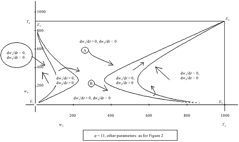
Figure 7. The graph shows that if j is rather high (11), the area of combinations of wA and wB which cause the growth of both the variables is divided into two parts.
ferent productive capacities (HB < HA), compete in a scenario characterized by a high propensity to the relocation of investments, unless the less productive system is initially more developed than the other system (evolutionary trajectory A in Figure 7), it can carry on at very low levels of GDP for a long period of time (evolutionary trajectory B in Figure 7).
4. A Model with Three Components
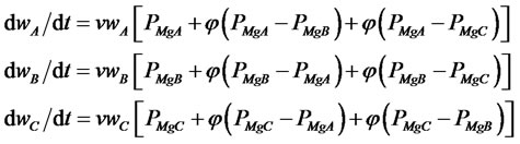
We present below a configuration of model 3.11 with three components:
 (4.1)
(4.1)
The numerical simulations carried out with this model (figures 8-10) provide us with some information.
Figure 8 shows the evolution of wages of three areas, a central area (A), with HA = 1333.3333, and two peripheral areas, both with H = 1200 (HB = HC = 1200). The targets of peripheral areas, however, are different, because only the target of zone C is lower than the target of zone A12 Area C, which in the simulation has lower initial values of wages and employment, remains depressed for a long time, but when it finally emerges, it surpasses area B (which has higher expectations, due to its cultural and/or political ties with area A). During its rise, due to investments flowing from A and B, it causes a temporary depression in wages and employment of these two areas.
This depressive effect can also be very strong if the system is very open and investment flows are highly sensitive to the differences of profitability, as is shown in Figure 9, which shows a situation like that of Figure 8, but with a value of φ far higher (φ = 11).
Figure 10, finally, shows the eventuality that the whole system, composed of areas A, B and C, starts from an initial condition with low wages and a low employment level, but with high capital mobility among the various areas (φ = 11). It is interesting to notice that in this case the best expectations of area B can cause a very long depression in this area.
5. The Role of the Interest Rate (Endogenous)
So far we have been examining a scenario in which investments are prevalently direct, without considering the possible differences and/or variations of the interest rate. We have already mentioned, on the other hand, that it is in those countries and regions which are more in need of loans that the interest rate is often higher.
The problem of the interest rate, on the other hand, is strongly debated, above all on the issue of its exogeneity or endogeneity.
By means of the model presented in our work, in this section the interest rate will be made endogenous13, so as to verify which factors can cause a persistent difference between the interest rates applied in differently developed regions.
We have seen (Formula 3.6) that the equilibrium wage grows in proportion to productivity (expressed by H) and that it is suffers a negative influence from both the interest rate and the target wage T. On the other hand it can be presumed that in regions of the same state it is difficult to differentiate wages and this can be one of the reasons why there is a strong incentive for irregular labour in backward regions, also and above all for the purpose of defending the capital yield.
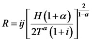
In our model the rents (R) obtained by financers are i w N (where N is the number of workers and w N is therefore the amount of wages: we have assumed, in fact, for the sake of simplicity, that work is the sole productive factor in which monetary capital is invested) and therefore, considering 3.3 (N = j w), in the hypothesis that the interest rate is endogenous, we have:
 (5.1)
(5.1)
Figure 11 shows the combinations of interest rate and amount of rents depending on different values of α, which here is assumed as an independent variable.
The figure is composed by two graphs. The first shows the relation between the values of α and those of the interest rate. We can see that the latter decreases when the former grows until it reaches a critical value at which the equilibrium wage (w*, i.e. the wage which maximizes profits) equalizes the target T. A further growth of α, since it cannot cause an increase in effort, which is already at a maximum, determines a lower than expected increase in rents. In this case, in fact, the equilibrium interest rate will be the one that allows the condition w* = T. This will be realized for a rate that is above the rate which could maximize rents if the output of a single worker could be exceeded H.
The amount of rents is shown in the left graph, which shows the relation between them and the interest rate. We can see that the relation is direct for relatively low values of α, then it becomes negative and finally it becomes direct again for values of α higher than that for
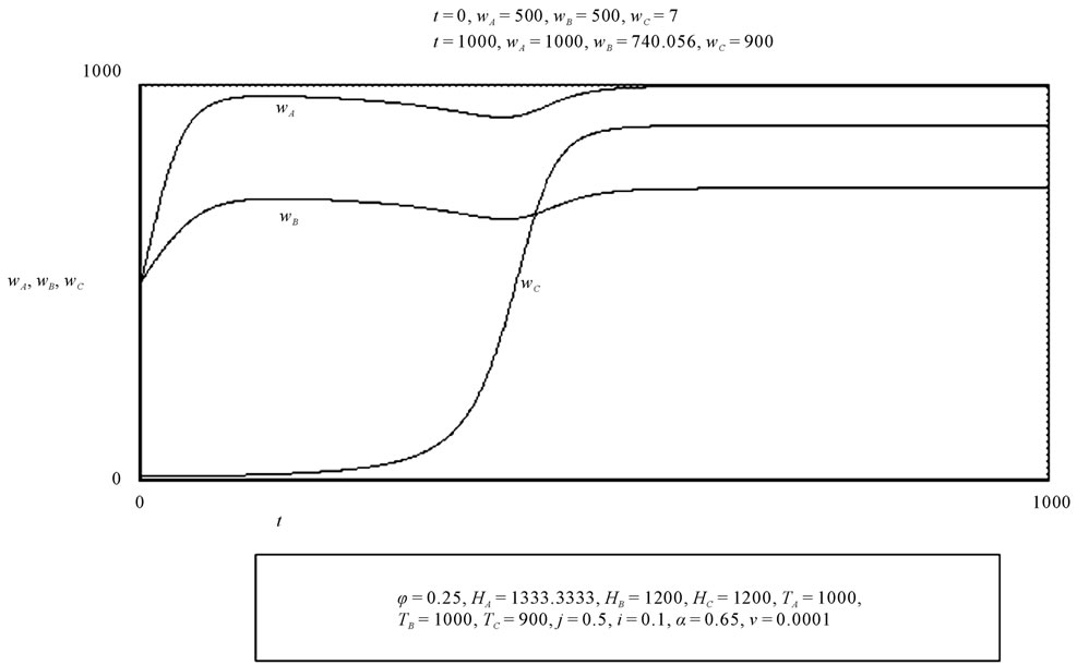
Figure 8. This shows the evolution of wages (and indirectly of economic development) in three areas, A, B and C. The perspectives of development are greater in region A, due to its centrality. The wage to which workers of area B aspire is higher than the wage desired in area C. The final result is favourable to the workers of area C.
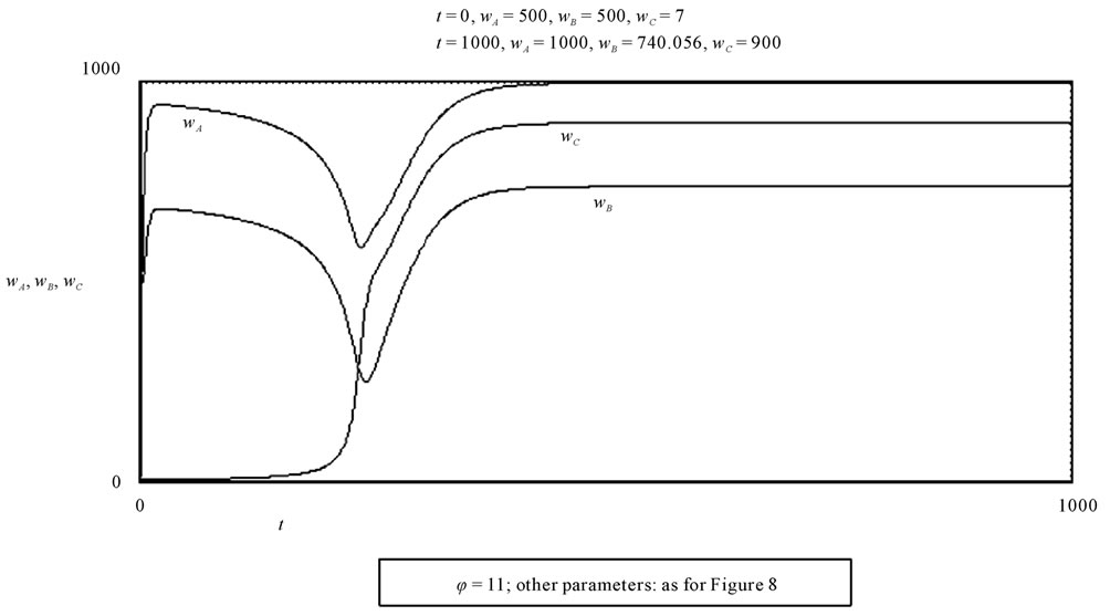
Figure 9. The graph shows how high values of j (re-localization rate), during the emergence of an area C, entail the fall of wages in areas A and B.
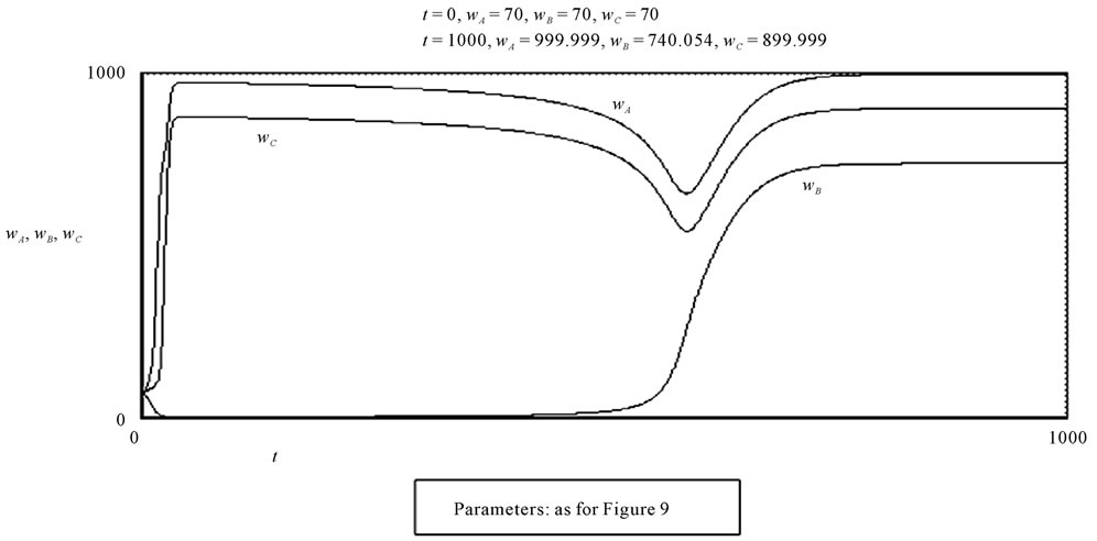
Figure 10. The graph shows the evolution of wages (and indirectly of the development rates) of the three areas A, B and C. The initial values of wages are the same and are rather low and the relocalization propensity is very high (φ = 11). The wages of area B, in which workers have higher wage expectations than workers of area C, fall and remain low for a long time.
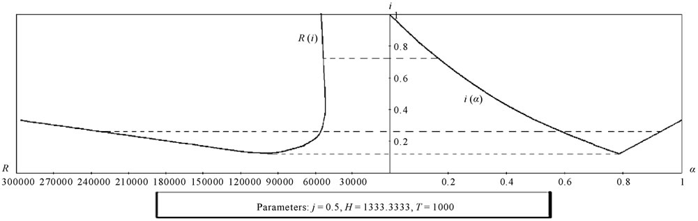
Figure 11. The right panel shows the relation between the interest rate i (dependent variable) and α. The interest rate, growing α, decrease to a minimum value at which the real wage is equal to the target T. Futher increases in the value of α do not increase the effort, which is already full, and therefore revenues grow less than we might expect. The left panel shows, on the other hand, the variation of revenues R as a function of i. For low values of α the relation between i and R is direct. It then becomes negative and then again direct afterwards the real wage equals T.
which the effective equilibrium wage equalizes T. We must remember that in our model α is related to effort. Low values of α indicate that the effort has relatively little influence on productivity (for example due to advanced technologies): in fact, low values of α imply that workers can maximize their production with a little effort. If this is the case, rents can be lower, although rates are higher14,15. Even for high values of α, however, which denote a great importance of effort, presumably associated to backward technology, rates can be quite high.
Obviously financiers will tend to maximize rents. Due to the fact that they can fix the interest rate, in the end they will absorb all the profits16. The wage paid by entrepreneurs will therefore not be that which maximizes profits, but that which does not cause loss: the profit curve, in dependence of wage, will be totally below zero, except in its peak. This is justified by the fact that in our model we have assumed that producers depend totally on financiers for their investments (they do not have their own capital): the final result is that they are remunerated only by the executive salary.
This extreme situation denotes that there is a natural conflict between finance and the real economy, between financiers and producers.
It is interesting to look at the scenario determined by rather low target wages (for instance, in the Third World). As we have seen above, low target wages cause higher equilibrium wages (but not greater than T). Beyond a certain limit, however, we have a situation like the one we have just seen: if w and T assume the same value, eventual ulterior reductions of T cause an increase in the interest rate. In fact if T is very low, the inversion point of the curve i(α) represented in the right graph of Figure 11 approaches the origin of the axes and beyond the inversion point the interest rate grows far more quickly (see Figure 12, with T = 300).
This is then a scenario in which direct investment (from external areas) is certainly greater than bank loans to local firms.
This scenario is no different from that exhibited by the real world. As noted by Spratt [17], the liberalization begun under President Reagan led to a far greater rise in interest rates than expected, especially in the poorer countries. Spratt also notes that, contrary to the predictions of orthodox economic theory, many studies have shown that growth in real interest rates has often led to a fall in rates of accumulation.
Examining the evolution of financial flows in the last two decades, moreover, it can be seen that these flows, once again contradicting the predictions of advocates of liberalization, did not exhibit a clear trend, but rather a cyclical pattern [17], with an alternation of increases and decreases. The picture begins to cause concern if we exclude direct financing.
With this exclusion of direct financing, in fact, financial flows between developed areas and emerging areas have not only fluctuated, but have periodically changed direction revealing, ultimately, a substantial net outflow from emerging countries to developed countries [17]. These results are affected, in actual fact, by the Asian crisis of 1997-1998 but, as Diaz-Alejandro [18] has stressed, a clear effect of liberalization has been, precisely, the increase in the frequency and intensity of financial crises, especially in less developed countries.
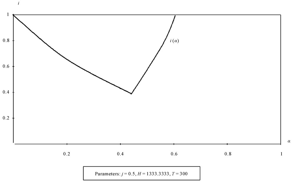
Figure 12. The graph shows the relation between a (independent variable) and the interest rate i. Unlike the case shown in Figure 11, the value of the wage target T is much lower: 300 as opposed to 1000. The turning point of the function i(a) is closer to the origin of the axes and the right arm of the curve is much steeper here than in the graph of Figure 11.
This is a result which cannot be taken into consideration by the simple model presented here, built without taking into account the “humours” which, according to the most recent research (on this, see Buchanan [19]), greatly affect economic life. However, after excluding direct financing, the prevalence of financial flows from the emerging world towards the developed one, despite their variability cycle, can be explained by the model presented here, by means of factors that might be called “rational”, since they are linked to the pursuit of maximizing the revenue of financiers.
6. Results/Analysis and Conclusions
We have seen that if direct investment flows are too intense, they can cause sudden reductions in wages (and employment) in the areas they start from and that such reductions can sometimes last a long time. The investments can flow from the centre to peripheral countries (if the target wage is quite low in these areas) and in the opposite direction. In any case the workers’ only option is to accept or, if they have the opportunity to migrate, to reject the labour conditions which maximize the profits of the financiers.
Moreover, in the peripheral areas the interest rate might be higher than in central areas, thus impeding local enterprises which in many cases are presumably still small and therefore not able to make full use of direct financing. By means of the endogenization of the interest rate, our model describes a prevalence of indirect flows (i.e. by means of bank intermediation) from peripheral areas towards central zones, also showing the existence of a trade-off between financiers and entrepreneurs. All these findings are in line with various empirical studies which have shown an increase in rents at the expense of wages, an increase which certainly did not favour employers.
Obviously our analysis does not necessarily mean that a peripheral area is destined to remain so. We have assumed, in fact, that the polarization is determined by differences in production costs within a system, for a given product or service. It is therefore obvious that this is true for one or even for many products (due to agglomeration economies), but it is always possible that an area which is peripheral for some functions, may become the centre for some other functions, and this is so especially in a world which is increasingly oriented towards a more complex organization.
Specialization may therefore seem a solution to the problem posed by the dynamics of peripheralization. It should be added that in our model local productivity (H) has been considered constant in the various simulations. We could rightly assume, on the other hand, that H grows if the size of the economy increases (due to agglomeration economies), and then, in the model we propose, H increases if local wages grow, and this would probably accelerate the convergence. A full convergence of the values of local productivity, however, is not possible, at least for most products, due to geographical differences across regions (in terms of resources, climate, communications with other areas, topography, etc.). Even if these differences appear less and less influential, they lead however to an inequality in opportunities: in an increasingly competitive world, this can play a significant role. Globalization in fact increases opportunities, reducing the importance of physical conditioning, but for this reason it generates global competition, reducing the possibility of carving out inviolable niches.
7. Acknowledgements
We thank Giulia Urso (University of Salento) and Joan Mc Mullin for revising the English text, and Guglielmo Forges Davanzati (University of Salento) for some useful suggestions.
REFERENCES
- M. Ravaillon and S. Chen, “China’s (Uneven) Progress against Poverty,” World Bank, Policy Research Working Paper, Article ID 3408, 2004.
- C. Calderon and L. Liu, “The Direction of Causality between Financial Development and Economic Growth,” Journal of Development Economics, Vol. 72, No. 1, 2003, pp. 321-334. doi:10.1016/S0304-3878(03)00079-8
- J. Schumpeter, “The Theory of Economic Development,” Harvard University Press, Cambridge (Mass.), 1934.
- J. H. Lopez, “Pro-poor Growth: A Review of What We Know (and of What We Don’t),” World Bank, Washington DC, 2004.
- R. McKinnon, “Money and Capital in Economic Development,” Brookings Institution, Washington DC, 1973.
- E. Shaw, “Financial Deepening in Economic Development,” Oxford University Press, Oxford, 1973.
- G. A. Epstein, “Rentier Incomes and Financial Crises: An Empirical Examination of Trends and Cycles in Some OECD Countries,” Canadian Journal of Development Studies (with Dorothy Power), Vol. 24, No. 2, 2003, pp. 229-248.
- G. Krippner, “What is Financialization?” University of California, Los Angeles, 2004.
- G. A. Epstein, “Capital Flight and Capital Controls in Developing Countries,” Edward Elgar Press, Northampton, Forthcoming, 2004.
- T. I. Palley, “Financialization: What It Is and Why It Matters,” Working Paper No. 525, The Levy Economics Institute and Economics of Barde College, New York, 2007.
- S. Andriani, “L’ascesa Della Finanza. Risparmio, Banche, Assicurazioni: I Nuovi Assetti Dell’economia Mondiale,” Donzelli Editore, Rome, 2006.
- A. L. Paolilli, “Development and Crisis in the Late Middle Ages: The Role of Trade,” Journal of European Economic History, Vol. 34, No. 3, 2005, pp. 687-717.
- A. L. Paolilli, “Development and Crisis in Ancient Rome: The Role of Mediterranean Trade,” Historical Social Research, Vol. 33, No. 4, 2008, pp. 274-289.
- S. Andriani, “L’ascesa Della Finanza. Risparmio, Banche, Assicurazioni: I Nuovi Assetti Dell’economia Mondiale,” Donzelli Editore, Rome, 2006.
- J. Schumpeter, “Theorie der Wirtschaftlichen Entwicklung (English Edition: “The Theory of Economic Development”),” Harvard University Press, Cambridge, 1934.
- T. B. Veblen, “The Theory of Business Enterprise,” Scribner’s, New York, 1904.
- S. Spratt, “Development Finance. Debates, Dogmas and New Directions,” Routledge, London and New York, 2009.
- C. Diaz-Alejandro, “Good-Bye Financial Repression, Hello Financial Crash,” Journal of Development Economics, Vol. 19, No. 1-2, 1985, pp. 1-24. doi:10.1016/0304-3878(85)90036-7
- M. Buchanan, “The Social Atom,” Bloomsbury Press, New York, 2007.
NOTES
1The concept that financial institutions can have a crucial role in economic development is not new. In particular Schumpeter [3] pointed out that they facilitate the introduction of innovations which lead to higher productivity without a prior saving, by means of a process of creative destruction.
2While the first approach assumes that economic development is favourable to the poor if their income grows, in relative terms, more than the per capita income (within this approach there is a more radical position which considers development favourable to the poor only if there is an absolute reduction of poverty), the scholars, like Ravallion and Chen [4], who follow the second approach, find it enough that the development increases their average income, without considering the level of social inequality.
3In some papers about the Middle Ages and Ancient Times [12,13] it has been stressed that two other periods characterized by a strong economic development, i.e. the Roman age and the Commercial Revolution of the Late Middle Ages, were accompanied by a great expansion of money (and, at least for the Middle Ages, by credit), and that in both the cases a monetary crisis, causing a partial regression to barter and a subsistence economy, significantly accentuated the successive economic decline.
4The function used to describe the direct relation between wage and labour productivity is of the Cobb-Douglas type, with decreasing marginal outputs.
5To obtain the value of w* we must rewrite 3.5 to show j and w:
0 = j {w [H (1 + α) (wα−1/Tα) − 2 (1 + i)]}. We can ignore the elements which are not in the square brackets, reducing the relation as follows: H (1 + α) (wα−1/Tα) − 2 (1 + i) = 0. We have wα−1 = 2 (1 + i) Tα/[H (1 + α)], from which, elevating all to 1/(α − 1), we obtain 3.6.
6To obtain the value of H*, the first step is to equalize w and T in 3.5, assuming w = T. We can then simplify 3.5, as follows:
0 = H j (1 +α) – 2 j T (1 + i). From the last relation we obtain 3.7.
7The marginal profit is the increment, or the decrement, of the global profit depending on the growth of investment.
8Obviously the proximity should not be such as to suggest an imminent incorporation of the peripheral zones into the central area, otherwise their very identification as a periphery would be challenged.
9We have regarded wA and wB as variables because their variation induces a variation of NA and NB and therefore of global investments.
10The coordinates of E4 are the same as the value of w* declared in 3.6. In fact the condition which makes both the equations in 3.11 equal to zero is the nullity of PMgA and PMgB.
11In this and in the other numerical simulations we have not set the duration of time unit, since this is not necessary for the purposes of this paper.
12A scenario of this type is the relation between Southern Italy or East Germany (area B) and the emerging economies (area C).
13We make the interest rate endogenous, i.e. we do not assume it as a given, but as an internal variable of the system described by the model.
14Financiers, therefore, may be interested in preventing productivity from growing too much (in accordance with the thinking of Veblen [16]).
15Remember that the higher the interest rates, the lower the actual wages.
16Our model provides outputs which look like the tendential fall of the profit rate, to the advantage of rents, already shown by Ricardo, although the mechanism which causes this result is not the one indicated by Ricardo.